Chapter 3 Scientific Laboratory Notebook
Dans les champs de l’observation le hasard ne favorise que les esprits préparés – In the fields of observation chance favours only the prepared mind. - Louis Pasteur
An integral part of any research lab is the lab notebook. Here, research refers to independent investigations as opposed to searching and reading work that has been conducted elsewhere. In this course, we will use notebooks in a similar way that scientists use them. For the purpose of this course the notebook can be an inexpensive composition book with 80 sheets, 9.75" x 7.5" in size, for example. It must be a bound notebook for reasons detailed below. The type of paper used in a is often also important. Acid-free paper will not deteriorate over time as fast as regular wood-based paper and it should not turn yellow.
Professional scientists use the to record events, such as experimental methods, file names, calculations, diagrams, sketches, ideas (creativity), suggestions, plans, observations, links, emails from collaborators, important plots and graphs, summaries, and abstracts, and important events.
Beyond that, the notebook provides a way to disseminate one’s own ideas deliberately. It can be thought of as a thinking tool to help fortify the thinking process. It also encourages writing, a skill that is strengthened by frequent practice. Sketching ideas, making drawings and diagrams is an essential part in the notebook. Visualization of ideas is an important aspect of communication and fosters collaboration between peers and teachers. In the end, the notebook will become an integral tool for writing reports, articles, and formulating a complete thesis. The lab notebook provides the historical (temporal) perspective, while a lab report, poster, presentation, or publication portray the logical flow of events. d
3.1 Organization
The organization of the lab notebook takes some practice. Here, the most basic structural elements for keeping a scientific notebook are summarized (Kanare 1985).
All pages in the notebook need to be numbered; also set page numbers apart from other numbers by encircling them; no page can be left completely empty - write "intentionally left empty" to fill any such page. You should keep close records of the dates and even the times in the day in some cases. Notebooks and log books should have a longevity of about 30 years or more. Therefore, use pens and paper that resist degradation. Use water, acids, and other common lab chemicals to try to wash off writing in order to test for the best pen to use. The notebook should also be bound (not spiral or loose-leaf), otherwise there is a chance that pages are removed or inserted. Pencils are not allowed, anything that can be erased leads to ethical problems. White-out cannot be used; only cross-outs are allowed, such that the text underneath is still legible.
The first two pages should be reserved for "Table of Contents" and "Projects" which you update with time and include the page numbers and date in three separate columns. Also make sure to include complete contact information, such that the notebook can be returned in the event that it goes missing.
Penmanship is crucial. The writing must be legible, clear, and each section needs a concise, descriptive heading. Headings include "Purpose", "Method", "Experiment", "Analysis", "Apparatus", … and should be used to delineate different parts.
Use acid-free glue or high-quality tape to insert paper snippets, print-outs, graphs, and other data into the lab notebook. The historical order is not interrupted. If the graph cannot be added at the moment, when the data is recorded, then no space should be kept for it. Rather at the later point in time, when it is added, the graph is pasted in the new empty space with a reference to the page number of when the raw data was collected.
Lab notebooks generally stay inside the lab and belong to the research laboratory. The lab notebook is separate and specific to each lab. It belongs to the lab director, who can inspect and verify the notebook periodically. The lab notebook should be stored safely.
Dates need to be recorded clearly (10/13/12 is not clear). The year always needs to be included using the full 4-digit representation. The month can be spelled out, if it is ambivalent. Due to data saving and ordering on computers, the recommended format is yyyy-mm-dd, or year-month-day representation.
Bad record keeping can have ill effects. In the worst case of disputes, credit of discoveries cannot be given.
The data is crucial to an experimenter and absolute and outmost care needs to be taken in collecting and storing scientific data. Data that is stored on computers must comply with a . This is a formal document that describes the process of securing and organizing lab data. It is a requirement for many grants, such as National Science Foundation (NSF), Department of Energy (DOE), or Department of Defense (DoD).
Data includes measurement points gathered using equipment, software
programs, models, reports, and publications. If the data is stored in
proprietary formats, it can cause problems at a later time. First of
all, some formats may no longer be supported or become outdated. They
may be operating system dependent. As a general rule, data should be
stored in text format, preferred format is CSV (comma separated files) or if the data is more complex in XML. The format (metadata) needs to be documented; i.e. the files should include consistent headers with units in one line and possibly follow a strict convention. If data is
acquired in a compressed or proprietary format, it must be converted to text format and stored along with the original data. The procedure of data conversion is part of the.
3.1.1 File Naming Convention
Slightly different conventions exist between labs. However, best
practice suggests that all raw data files are stored in one single
folder called RAW in a flat format (there are no sub-folders).
Therefore, the file names ought to be unique. The generation of is as
follows. Each raw data file name contains 6 parts: (1) the recording
date (yyyymmdd-), (2) the project name, (3) the instrument name,
(4), the main user’s initials, (5) the sample name, and (6)
extra description. An example would be
20140820-nmrlab-tg-PNMR-GL01-run1. In this case the sample name is
GL01 and the author’s initials are tg. The file name needs to be
recorded in the and the extension depends on the machine. In this
fashion, one RAW folder contains all data files and they can easily be
searched by date. In fact, if you look at your notebook, you should
almost be able to guess the filename from for the experiment performed
on a certain date. Alternatively, you could easily search for all files
that belong to the project called nmrlab or all files from sample
GL01. Typical instrument names include PNMR for pulsed nuclear
magnetic resonance, AFM for atomic force microscopy, and XRD for
x-ray diffractometer.
3.1.2 Notebook Organization
What are some good examples and traits of a successful lab notebook? It should include some of the following ingredients:
personal expressions, comments ("good sample", "worked well", "process is too long", etc.)
sketches, drawings, diagrams, processes
questions, predictions, and hypotheses
full sentences with reflections and analysis
detailed descriptions of the experimental procedure
Many keepers will also sign the page at check-out, or have the notebook inspected and signed by the lab supervisor.
You should acquire a style of notebook keeping that avoids making notes on loose paper, only to be recopied later. Your style of record keeping should be useful to others, therefore use legible writing, and complete accounts of your experimental procedure and details. For computer programs, include flow diagrams in your notebook. Keep your notebook in a well-protected space. Keep your audience in mind. For one, it will be yourself, you will want to write a lab report or thesis based on the measured results. Another person may be a peer who will continue measurements. Clarity in writing is important, some details may be clear at the moment, but will be in question later in time. It must be recorded to avoid confusion later on.
All information and data must be recorded unambiguously. Describe the conditions of the laboratory. Flexibility in the format should be used, however. Always include the leading 0 for numbers \(< 1\).
3.2 Evaluation
The evaluation of the lab notebook is based on the following criteria:
full name and department on cover
start date (and end date if full) on cover
first page: complete contact information, including email
second page: table of contents (will be filled in with time)
date and times are recorded, if other people helped take data, include their names
all pages are numbered; page numbers are circled
no pages are skipped (blank)
all dates are spelled out in format yyyy-mm-dd (include 4-digit year and order in this way)
use only pens (no pencils, white-out) that withstand water, alcohol stains and withstand time
use headers, organize whenever possible
include appropriate sections such as "purpose", "method", "results"
include complete record of experiments, use full sentences
include every filename of data that is recorded, or for programs that you write
filenames should be unique (NOT
experiment1.datortest5.dat) and inaccordance with Sec.3.1if graphs are taped, make sure they are well-taped, no post-its, loose paper
mistakes are never blacked-out or deleted with white-out, rather crossed-through, or if occurred in the past amended with a note (referring to the current page, where the corrected information is given)
In the event, that you discover, that past data was recorded incorrectly, make the amendments on the new pages (current time) and only add a reference to the current page number on the old pages. Do not change the past.
3.3 Notebook Examples
The content and organization between lab notebooks varies a lot. In fact, notebooks have personal and distinct character. You may also have seen bad examples, incomplete lab notebooks. Therefore, it is important to self-review the notebook, based on the organization and evaluation principles outlined in Sec. 3.1 and 3.2. It makes sense to also read and study notebooks from other scientists (Kanare 1985).
One famous scientist from the 19th century was Charles R. Darwin (1809 – 1882). His best known book is called "On the Origin of Species" (1859), in which he rejects some earlier concepts on transmutation of species. In the book, Darwin describes his voyage around the world and explains the origin of species through natural selection. He kept notebooks in order to keep track of events. Many of his notebooks are available online (http://darwin-online.org.uk/). A typical notebook was leather-bound and contained about 100 folios (leaf), effectively 200 pages. The table of contents was added to the front page for archival purposes. It was written in ink. In the text, Darwin states facts from other scientists and debates them in the text. He uses words such as "to my view" and questions like "Why would we have …". The Edinburgh notebook (1827) contains a lot of sketches. Darwin’s notebook B is particularly famous as it shows sketches between related species corresponding to the tree of life.
An extensive library of books exists for physicist Marie Curie (1867 – 1934) chronicling her life. She was awarded the Nobel Prize in physics for her discovery of radium. A few years later, she received a second Nobel prize in Chemistry. She was a brilliant and determined scientist, born in Poland, and worked in France. Her notebooks are kept in lead-boxes, since they are radioactively contaminated. Radium has a half-life of 1600 years after all. Notes over a three-year period from 1899 are available in the Wellcome Library in London. It contains notes of experiments on radio-active substances, and pen-drawings of the apparatus. Madame Curie included notes on setting up equipment, experimental conditions, and nice drawings of how electrical wires were connected. She also kept nice tables that interrupted the flow of text and equipment sketches. Interestingly, she noted strange observations – on thorium oxide activity decreasing with air flow in the ionization chamber - which were not published. Rutherford, a bit later, found the same and postulated the emission of radioactive gas by thorium oxide. She used lines to delineate experiments and separate portions.
Physicist Albert Einstein (1879 – 1955) known for his publications on special and general relativity kept good notebooks. The notebooks are available at http://alberteinstein.info/gallery/science.html. One notebook is particularly famous, it is the Zürich notebook written in 1912 – 1913, it contains both images, equations, sketches, and words. This notebook - subtitled "Notes for lecture on Relativity" - describes the fruitful phase of Einstein towards developing the general relativity (Straumann 2011). Note the page numbers are centered at the bottom of each page and surrounded by dashes, so that they are not confused with any numbers. He used dividing lines to separate parts. On page 38, he writes "lautet unsere Nebenbedingung", which is interesting because he uses the word "unsere" (our) to discuss his own work. In this case, "we" corresponds to the "royal I". Einstein used notebooks to jot down tidy and messy notes, some notes have annotations, some pages include calculations and some pages are crossed out, followed by "Nochmalige Berechnung" (Zürich notebook, p. 37) or new calculation. Most of the notes were not intended to be read by others (Janssen et al. 2007).
Another Nobel laureate who kept nice lab notebooks is chemist Linus Pauling (1901 – 1994). His notebooks are available online (http://scarc.library.oregonstate.edu/coll/pauling/rnb/); a total of 46 notebooks are available and the handwriting is particularly legible. He includes references to literature in his notebook. In the writing you find words that express his emotions, such as "a beautiful hemochromogen spectrum" (July 9, 1935). These words are perfectly acceptable in a personal research notebook, and give away success and failure, however, they are not to be used in publications or lab reports, where the text is devoid of emotional words. Indeed, the lab notebook is a subjective account that is translated into an objective narrative to be published. You may also note that times are included, such as "10 AM Sunday January 19, 1936" (Notebook 13, p. 47). In another example, you can see that Pauling singly and doubly underlines words to provide content. He also uses headers such as "Discussion" and indents paragraphs. You note on page 49, he writes "See p. 113 for correction". The practice with notebooks is to provide a historical account, therefore corrections cannot and must not be added to past pages. At one point, he writes "I have no explanation to this to offer.", which is a complete sentence rather than some shorthand.
Finally, physicist Richard Feynman (1918 – 1988) is known for his teaching style and contributions to quantum electrodynamics. Some of Feynman’s notes are available in the Caltech archives (http://archives.caltech.edu/). His notebooks contain lots of diagrams and sketches, ultimately culminating in what we know as Feynman diagrams. His idea of the notebook is that it slowly grows the knowledge from something fuzzy into something concrete. That demands sometimes an ability to focus and deliberately add careful notes over longer periods. It is another skill to practice, if you fully embrace and accept the benefits of notebook keeping.
In summary, these accounts show examples of lab notebook taking. In particular, you learned that full sentences are used in conjunction with date and time stamps, and header lines. Often, it is a subjective account with a personal style. The lab notebook plays an important role for any scientist, it protects the owner from (legal) disputes by keeping records and original work safe.
3.4 Trends
Scientific note taking has changed over time. In earlier times (17th century), some notes (Gallilei) were encrypted or distributed as anagrams to claim first authorship, but not to give away all ideas. Before typewriters, notebooks served the important task of organizing thoughts. More recently, electronic note-taking has taken foot hold (Giles 2012). Some researchers are using shared document spaces, such as offered by Google or through Dropbox. More specific solutions include LabGuru (biology oriented) or Quartzy (https://www.quartzy.com/). For large collaboration such tools may become important, although it is clear that they create an overhead, backup issues, extra costs, flexibility, and require maintenance by a supervisor. Still, taking notes in an acid-free notebook is common and standard practice and maintains the most advantages over long periods of time.
3.5 Scientific Research Publications
You will learn to read, write, and understand scientific , including research papers, dissertations, and M.S. theses. It turns out there are basic patterns that research papers generally follow. By reading scientific papers, you will become familiar with this specific structure. Writing reports allows you some practical experience with this style.
3.6 Literature Search
Science is an ever-evolving process. In order to start, you will need to obtain some background information about what experiments have been completed most recently and which theoretical models have been proposed and tested. There are many journals that publish results. The wealth of available articles may make it difficult for someone new to a field to find relevant information.
There is a procedure, which is detailed in an article by . It starts off by using a journal database. These journal databases are listed by the library under the subject. There are several websites that can be helpful in locating research articles:
In order to narrow your field, you may target specific journals, specific search engines, and relevance sorting. All three will be briefly described here. You may start your search in a specific journal. For the physical sciences a few peer-reviewed journals are the following:
Physical Review Letters (PRL)
Physical Review A,B,C,D,E (PRA,PRB,PRC,PRD,PRE)
Applied Physics Letters (APL)
Journal of Applied Physics (JAP)
Reviews of Modern Physics (RMP)
Europhysics Letters (EPL)
Nanoletters
Physics Today
The importance of a journal is generally denoted by an index called impact factor, a higher impact factor means more relevance. It is a bit controversial as to what it actually measures and there may be other tools to assess the importance of journal. The impact factor of a journal may change yearly. The impact factor of PRL is 7.3 (2009) / 9.2 (2021) and the impact factor PRB is 3.5 (2009) / 3.9 (2021), for example. When starting with a new topic, it is suggested to read "review papers" that give an overview of the topic and often cite important literature. You can then continue reading papers that are cited in this review article.
Expert readers in physics often read a journal article not in a linear fashion, but start by reading the title, the authors, affiliations, and the abstract. If the interest is awakened, then they quickly turn to the figures and read all the captions. Next, the expert readers often take a quick look at the summary or conclusive remarks, before turning to other content in the paper. The first and sometimes the first two paragraphs give you a review of previous work and motivations for the research. Therefore, as a part of the literature review process, after finding papers, focus on reading the first paragraph after the abstract and take notes of the motivation for the research.
If you begin reading articles, you should steer to the first two paragraphs. These paragraphs summarize the motivation for the specific background. Open questions and puzzles are often raised in these important paragraphs. Using pen and paper, find about 10 articles on a chosen topic and only read the first 2 paragraphs, then summarize the motivation for each article. You should get a good perspective quickly.
One product of research is a publication, such as research papers, theses, conference papers, presentations, and books. These research products are generally peer-reviewed before publication; i.e. experts in that particular field provide feed-back to an editor to keep standards in the field. Therefore, when you submit an article to an editor, you will need to have an author list of potential reviewers ready. For this purpose, you may make an author map using Web of Science (WoS): CSULB Library
3.7 Search Strategies
When entering a new field with a vast repository of journal articles and information, a strategy must be applied to find informative, reliable, and broad articles in the new field. Database engines can be used for this purpose. Always use the "advanced search" option, either in Google Scholar or Web Of Science searches. If you are unfamiliar with a topic and want to find out what has been published in this field, then start a search using the topic search field TS. For example, TS=atomic force microscopy, then sort your search by most citations. The most cited work generally can be viewed as being perceived as more relevant by the research community. Scan the 10 to 20 most cited works in the field and combine reoccurrences in the title. Then refine your search by limiting the journals, for example. Useful fields to refine your search are the title field TI, the published year field PY, or the journal SO. If you are interested in articles on nanotubes from CSULB, you could search for TS=nanotubes AND ZP=90840, for example. An article published in Physical Review Letters will be general and more readable than a more narrow journal. Sort again for most cited, or most recent articles. Once you find a few intriguing titles, read the introductions of several related papers while taking notes. At this point you should have general idea of the questions that arise in the field. Use this additional data to focus your searches and create a better picture of the research field and how to position your work within.
Several tools can be used for a reference manager. A simple tool is the add-on for Chrome browser called Zotero, which can also run as a stand-alone application. It easily integrates with LibreOffice Writer and LaTeXdocuments.
3.8 LaTeX
Most professional publishers use a compiler to create documents. Most commonly, this compiler is based on a language called LaTeX. Unlike traditional Word processing software, it is not a WYSIWYG (what you see is what you get) software. The idea is that the program takes care of all the formatting and you are solely responsible for the text and the graphs. Therefore, if you were to write a report, you could easily compile it one way (two-column format), and then compile it for another publishing style (double-spaced document). Often you will write several reports, so that you only need to worry about the formatting once; you can instead focus on the content more as you progress. Moreover, the compiler takes care of labeling figures, positioning figures, and referencing / citing.
Most physicists are familiar with LaTeX. The most common distribution is called MikTeX (http://miktex.org/) and can be installed on other operating systems. Additionally, an editor is used. For Windows, the editor that is preferred is called WinShell (http://www.winshell.de/), and for Mac OS it is TeXShop (http://pages.uoregon.edu/koch/texshop/). Since the installation may be troublesome for some users, there is an online version, which requires no installation and maintenance at all, called OverLeaf (https://www.overleaf.com/). In that case, you can register using your email. OverLeaf also makes many report templates available, so that you can quickly start with your report.
3.8.1 Getting Started with LaTeX
In OverLeaf, after login, you create a new project. You
can select a "blank" project or choose a template. You will have a
split screen, on the left are the files for the document, in the middle,
you find the code, and on the right side is the compiled document, which
you can download in PDF. Each LaTeXdocument has two sections, namely a
header and the document. In the header, you include the definitions,
usually, you don’t change anything after loading the template. The
second part starts after \begin{document}, see
Lst. ??. Your text can simply be inserted after
the command \section{Introduction} and before \end{document}. If you
start with a blank document, or use your own compiler, then the code in
listing ?? will be a good starting point.
Use the \section{} command to generate title headings, which are
automatically numerated. If you want to avoid the numbering, then add *
after the word \section, such as \section*{Introduction}.
Physicists and mathematicians particularly use equations, which are
easily typeset using dollar signs. The dollar signs surround the
mathematical text and also parameters, so that they are cursive in the
text. For example, an RC circuit would have the time-dependent electric
potential \(V(t)\) typeset by $V_0 e^{-t /(RC)}$ which shows as
\(V_0 e^{-t /(RC)}\). As you can see, the underscores create subscripts,
and carrots are used for superscripts. The curly brackets define, which
part to superset. Use \sin \theta for functions to display
\(\sin \theta\) and note the slash for the sine function. Without the
slash it would not be a function, but the product of three variables.
\documentclass[aps,prb,amsmath,amssymb,reprint]{revtex4-1}
\usepackage{graphicx}

\begin{document}
\title{My Title}
\author{Your Name}
\affiliation{Department of Physics and Astronomy,
California State University Long Beach, CA 90840}
\date{\today}

\maketitle

\section*{Introduction}
Your Text
\bibliographystyle{plain}
\bibliogrpahy{myBib}

\end{document}
In Lst. LaTeX Example, the document class is RevTeX, which
includes many useful macros for the Physical Review journals. One such
macro is useful to include an abstract. You simply surround the abstract
with \begin{abstract} and \end{abstract}, and it will be formatted
properly. The same can be done with the acknowledgement. Towards the end
of the document, use \begin{acknowledgement} and the corresponding end
command.
If you have not compiled a document in LaTeX, try to compile
Listing @ref(#list:LatexSample) in OverLeaf, omit the \bibliography for
now, as it will be explained later. A video may help creating the first
document: http://tinyurl.com/FirstLatexPgm. An excellent and through
introduction in 2.5 hours is found in the CTAN short introduction:
https://ctan.org/pkg/lshort-english.
3.9 Bibliograpahy
Researchers often write extensive documents, such as reviews or grants,
with 100 or more citations organized in the or section. The organization
of those references and documents becomes paramount in these
circumstances and the same process can be used and practiced with
smaller documents (Duong 2010). The free multi-platform utility
helps you collect, organize, cite and share research articles. It can be
installed as a stand-alone application and minimizes the workflow. Next
to the URL in the web browser the Zotero button will appear after
successful installation. Pressing this button will export the complete
citation information to the Zotero database. In Zotero, you can
right-click the library and Export Library … in the
format "BibTeX" to a file called "myBibtex.bib" in this example that
can be directly included in a LaTeX document, see
Listing ??. In addition to the filename, you also
need to specify a style for the bibliography. The style can be
customized, if needed. In the example of
Listing ?? the style "plain" is used. The \nocite
command makes sure that all citations in the included file are listed.
\documentclass{article}
\bibliographystyle{plain}
\begin{document}
\nocite{*}
\bibliography{myBibtex}
\end{document}
Depending on the compiler that you are using (TeXShop on Mac, WinShell on Windows), you may have to do a separate compilation for the BibTeX file, and compile the LaTeX file twice.
The location of the citation in the document is important. It appears at
the end of the sentence or after the quotation, text that is borrowed
from the cited document. The command \cite will place the proper
citation in place.
An additional feature is implemented by installing the "Better BibTeX"
add-on (https://zotplus.github.io/zotero-better-bibtex/) in Zotero. It
will auto-sync a library, so that constant exporting is not needed.
Secondly, selecting a reference in Zotero and using the copy command
will generate the proper \cite command.
3.9.1 Zotero Activity
In this , you will learn how to cite articles. You will get familiar with the reference program (https://www.zotero.org/), and learn how to format references in different styles using . You will also learn about how to search for articles using . Your final work should list at least 5 review articles.
In the first part, start the application. Zotero is a program that is available on multiple platforms and allows you to collect, organize and cite research articles and resources easily. It will be particularly helpful, once you write longer articles, thesis, or dissertation.
Determine the research topic for the search
Start the program Zotero. If it is not installed, then install it from the website: https://www.zotero.org/ (use Chrome browser and add the Zotero extension).
In Zotero, click on the My Library folder and create a New Collection named after your research topic.
Follow this example to find research articles on your topic.
Go to the Library page, and click on Databases by topic, then select "Physics & Astronomy".
You can choose any option, but for the purpose of this tutorial, we will continue using the "Web of Science" (WoS) database. If you access the database outside CSULB, you will need to use your studentID and password to use the service.
Choose Advanced Search
Use the field tags to make a search, such as TS=YOURTOPIC AND TI=REVIEW, where you replace YOURTOPIC and then sort by citations. To first order, the most cited articles are important to the field, if the search returns a large number of articles.Try out different search strings to find good review articles on the topic of Nuclear Magnetic Resonance.
Choose an article and make sure that the abstract is interesting and really is a review paper on the topic. Tweak the search, if needed.
Click on the page icon next to the star icon, see Fig 1.1.
Repeat process and add more references to your Zotero database.
You may also add a book on the topic.
The Zotero reference managers allows you to quickly capture references from a) the browser by simply clicking on the book-shaped icon next to the star bookmarking icon. b) ShareLatex has an upload feature to add the bibliography file that you (c) export from Zotero in format. It is useful to sometimes save in "Western" format.
Now returning to Zotero, right-click on your collection and click on Export Collection, see Fig. 1.1 c). The data is saved in a file that supports . It should have the ending .bib. Remove any spaces, underscores, and other strange symbols from the filename, as this could spell trouble later.
Now that the data has been exported, use a browser and open a new project in ShareLatex.
Go to OverLeaf.com
Login to your account (or make a free account, if needed).
Click on New Project (blank project) and call it research topic or similar.
Hit the Upload button, see Fig. 1.1 b), and upload the file
Before
\begin{document}write\bibliographystyle{plain}…Before
\end{document}write\bibliography{Topic.bib}(Note .bib extension is not necessary, but can be added, no spaces are allowed inside curly brackets.Make sure that the bib file has no spaces, if so, replace with dashes.
Include all members’ name in the
\authorargumentChange the title, and add some text for explanation of the document. Use the command
\nocite{*}somewhere, so that all references will be added.Add at least one citation directly, using the command
\cite{name}, the name of the citation is in the bib file after@article{Change the style of the bibliography from "plain" to something different.
Explore what difference the command
\citeAmakes.Download and save PDF document.
3.10 Report Structure
Each journal requires a specific style and that includes font size, graph quality, figure numeration, etc. The website for the journal denotes weather articles can be submitted in both Word format and/or in LaTeX format. LaTeX(note that the last letter is a Greek \(\chi\) and not to be confused with the Latin letter "x") is a popular format for articles and books. It is not a WSYWYG (what you see is what you get) format like Word, but rather needs to be compiled into PDF or postscript format before it is distributed. The LaTeX format is very flexible, since the compiler takes care of table of contents, page numeration, page spacing and style.
For example, there is a LaTeX template to write a CSULB M.S. Thesis, see the resource page on the physics home page (http://www.csulb.edu/depts/physics/resources/thesis_resources.htm). Once you insert the text, it will compile and produce a document that complies with the specific CSULB library standards. It will also generate a table of content and list of figures and tables.
A scientific paper, M.S. thesis, or Ph.D. is generally divided into 7 parts, each part will be explained in detail in the following:
Header
Introduction
Experiment
Results and Analysis
Conclusion
Acknowledgments
Bibliography
Header The header includes a title, authors, author affiliations and an abstract. The needs to be informative and necessarily reflect the goal of the experiment, but rather the result. The abstract contains all the information and main results and important conclusions of the paper. It is a quick way for a reader to get an idea of whether the article is of interest. A typical abstract has around 100 words and it is always a single paragraph.
Introduction The introduction provides sufficient background information and motivation to draw the reader in. Generally, this part will convince the reader that this particular research is worthwhile. Often conflicting models are described, advantages to certain techniques discussed, and the rationale for this experiment discussed. Only background information pertinent to the experiment should be provided.
Experiment The experiment describes the materials and method used. It should include the assumptions and background information of how samples were prepared, etc. The methodology is described, such that a reader would have sufficient information to duplicate the experiment and find the same results.
Results and Analysis The most important section contains the results of the experiment and their analysis. This section should include the necessary figures, graphs, and tables with captions to support the findings. The data of the graphs should be described and the implications discussed. Often, the results are compared to other similar research.
Conclusion This last short section summarizes the work and focuses the readers on the important findings without going into the details. It may reflect on special implications.
Acknowledgments This section acknowledges the funding sources, help with measurements and extra support from people who are not authors. This could refer to preparation of special substrates, the help with a particular measurements, or insightful discussions of the results and analysis with a peer.
Bibliography Previous research results should be cited throughout the text (except abstract) with the references listed here. Typical 3-5 page papers have 10-30 references, whereas M.S. thesis have 25-50 references and Ph.D. theses usually have over 100 references. The bibliography contains authors, journal name, journal volume, issue number, page number, and year of publication at the minimum. Sometimes, it also includes the title of the paper. Websites are not good resources for citations, as they tend to change, get modified or deleted. Whenever possible, reference to scientific literature should be made.
Other important restrictions include adherence to page limits, proper numbering schemes of pages, tables, and figures, page limits, and proper formatting of graphs. Each table and each figure requires a caption explaining the main parts of the table or graph.
3.11 Units
In physics, the units of choice are based on the Système International
(SI) units. Other common unit systems are the cgs system, which is based
on centimeters, grams, and seconds; it is particularly popular in
magnetism. Reports should exclusively use SI units with a few
exceptions, which are for temperature, where degrees Celsius () are also
used. Note that the units are not spelled out, as in the following
sample sentence: "The measured time constant \(\tau = 52 \pm 3~s\)". You
would not write out the word "seconds". In LaTeX, units are easily
integrated in the package siunitx, which is loaded with the code in
Listing ??. The command \SI uses two inputs, the number, and
the units; you can use engineering notation for the number as shown in
the example.
\usepackage{siunitx}
    \begin{documentclass}
    \SI{4e-6}{\meter}
    \SI{4.2e-6}{\micro\meter}
    \end{documentclass}
3.12 Presentations
Communication is a skill necessary in science. Research becomes the good of everyone; therefore dissemination is an important step of the research process. A presentation reaches a particular audience. The presentation should convey a particular message. This message is presented in the form of a logical story. There is a particular flow to this story.
The first slide is the title page, of course. It contains the carefully selected title, which should reveal the core of the message that you are going to present. It also has your name, your mentor’s name, and other contributors. Equally important the funding source is also listed.
All slides should use a font size that can easily be read by the audience. A minimum font size of 24 is recommended. The type of font is also important. In print, a serif font is commonly used, but for slide presentations, the font ought to be sans-serif, such as Arial. Finally, the color contrast must be good.
The second slide is very important; it needs to capture the audience and explain why they must be interested in your story. This slide includes the motivation for the research and makes a compelling case. It should provide enough context to make the specific research necessary. Starting with a broad point of view that includes all audience members. The broad picture is quickly focused towards the topic of interest. A relatively simple way to improve the motivation part is to notice that the first paragraph of most journal articles, but in particular PRL articles, are dedicated to integrating the larger picture.
The following slides tell the logical story, so throw out parts that do not belong into that story. Slides should mostly include images, photos, and diagrams that complement the speaking portion. The slides should stay up sufficiently long. Do not include details on the slides that you will not discuss. Do not go back to previous slides. Avoid full sentences and text on slides as they lend to reading the slides. If necessary, repeat the slide in the deck, however, form the story so that it logically progresses and presents evidence supporting the message that you want to convey. The title of the slide - if there is a title at all - should express the message not the content; i.e. it should not be results, rather spin-lattice relaxation.
Good advice is to only include material on the slides that you are going to cover and to avoid using the whiteboard, or moving backwards in slides. That is where practice of your slides and your story comes in. Provide an accurate representation of your work and the work of others; i.e. only include graphs, photos, or diagrams that are not copyright protected and include a clear reference at the bottom of the page. It is a common practice to have a summary or conclusion as the last slide. The special vocabulary required in your talk needs to be explained carefully and used consistently.
Graphs should have clear labels and units and they must be pointed out in the talk. Data tables are not effective.
Finally, it help to give the presentation in professional attire and to speak clearly and hold a laser pointer firmly (two hands). Avoid making jokes and side remarks as those should only be given by the most practiced speakers.
3.13 Data Analysis and Graphs
Modern data sets are large, so software must be used for analysis. Open-source software tools are particularly enticing. While plotting software, such as GnuPlot provide flexibility in making modern graphs, a more comprehensive plotting software is Python or the R Project, which run on many platforms. The R project can be used for batch data analysis, data fitting, modeling, and graphing. The language is most similar to MatLab and has many packages that extend its functionality. To follow this tutorial, you will need to install the R environment (https://www.r-project.org/) and RStudio (https://www.rstudio.com/), which provides an open-source graphical interface for R. Alternatively, it is possible to run R in the cloud, see for example RStudio Cloud (https://rstudio.cloud/).
In language, data is processed in so-called data frames. A data frame is
similar to a table and contains many labeled columns, which have data
stored in rows. A data column is generated from a vector using the
command c(). As an example, we will make a plot of the average
temperatures of Long Beach.This data frame has 3 columns, called month,
TL and TH. Note that the colon makes a sequence of numbers from 1 to 12
and stores it as a vector.
T.high = c(20,20,20,22,23,25,28,29,28,25,22,19)
T.low = c(8,9,10,12,14,16,18,18,17,15,10,8)
month = 1:12
data = data.frame(month=month, TL = T.low, TH = T.high )
Here is the code to make a plot using the package ggplot, which you
can install with the command install.packages('ggplot2').
Additionally, we are calculating the medium temperature by adding a new
column to the data frame called Tm. The aesthetics in ggplot defines
the x and y variables of the plot, which are month and Tm. Since the
label of the y-axis requires a superscript, an expression is used. The
last part chooses the number of breaks along the x-axis, in this case 6.
library(ggplot2)
data$Tm = (data$TH+data$TL)/2
exp.Temp = expression(paste("T ("^o,"C)"))
ggplot(data, aes(month, Tm, ymax=TH, ymin=TL)) +
  geom_point(size=3, color="blue") +
  geom_errorbar(color="blue") +
  theme_bw() + ylab(exp.Temp) +
  scale_x_continuous(breaks = seq(2, 12, 2))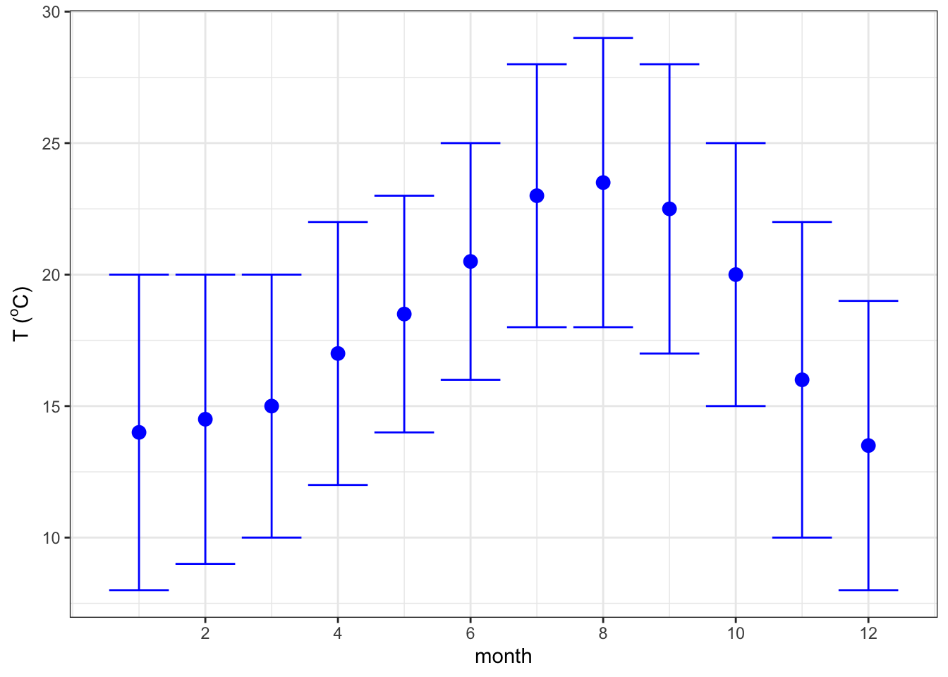
Figure 3.1: Basic graph of the temperature change
The resulting plot is shown in
Fig. 1.2. It can be saved with the command
ggsave('graph.png') in R.
Average high and low monthly temperatures in Long Beach, CA as plotted in R.
The following example (graph shown in
Fig. 1.3) demonstrates making a quick graph
from data collected on the Rigaku Smartlab x-ray diffractometer. The
diffractometer saves files in the RAS format, which can be opened with a
text editor. The data is read from the raw file with the
command read.csv. The header lines are automatically ignored as they
start with a comment symbol. The third column V3 is deleted, as it is
not needed here. Next, the columns for data frame d are relabeled with
names. In order to express Greek symbols in the x-axis, the command
expression is used. It also allows to include superscripts with the
symbol ^ and subscripts by enclosing the subscript in square brackets
([0]).
::: Shaded \[code:xrd_reading_example\]
# devtools::install_github("thomasgredig/dataLabManual545")
library(dataLabManual545)
data("AirPassengers")
# fname = "~/RAW/Ld20160514.ras"
# d <- read.csv(fname, header=FALSE, comment.char= "*",sep=" ")
# d$V3 <- NULL
# names(d) = c("TwoTheta","I")
# exp.TwoTheta=expression(paste("2",theta," ("^o,")"))
# ggplot(d, aes(TwoTheta, I)) +
#   geom_line(col="red") + theme_bw() +
#   scale_x_continuous(limits=c(5,30)) + scale_y_log10() +
#   xlab(exp.TwoTheta) + ylab("I (a.u.)")
The following is the result of the code on page loading and displaying x-ray data. The spectrum shows the Bragg-Brentano scattering from iron phthalocyanine powder.
3.14 Fitting of Data
The prevalent theme in physics is to make predictions based on a model. The experiment allows us either to confirm the predictions through strategic measurements, or to modify and extend a model. In this process, data is collected, graphed, and then compared with the model. Ideally, the model would quantitatively predict the experimental data. In practice, however, there may be some adjustable parameters that need to be fit. Therefore, is a common and useful practice.
A simple way to fit data is to linearize the experimental data, so that
the fitting parameters are either the slope or the offset of a linear
equation. A transformation of variables is done, so that the transformed
equation has the shape of \(y(x) = A + Bx\), where \(B\) is the slope and
\(A\) is the offset. By plotting the data in the transformed variables, a
ruler can be used to determine the fit parameters \(A\) and \(B\).
Alternatively, a program is used to help you fit the data, generally
using a non-linear least square fit. In R language, the function lm is
used to get a least-square linear fit.
As a practical example, if your data has the form of an exponential decay, such as in \(M(t) = M_0 \exp \left( -t / T_1 \right)\), then linearization would occur in the following way:
\[\ln \frac{M(t)}{M_0} = - \frac{1}{T_1} t\]
we have introduced a new variable \(y \equiv \ln M(t) / M_0\) and the running variable \(x \equiv t\) is the time. The offset would represent the amplitude of the exponential decay \(A = \ln M_0\), and the slope of the linear equation is equal to \(B = -(1/T_1)\) in this representation.
The following example provides code to make a fit using R. In the first
part, the data is loaded from a file generated by the Tektronix , which
is in a comma-separated format. The command to load the data into a data
frame is called read.csv.
library(dataLabManual545)
data = dataNMR
This data frame contains two columns labeled time and V, which
contains the time in units of ms and the electric potential measured in
units of V. A graph is generated by first invoking plot to generate
the data points. A second layer is added with the command points in
order to highlight the data points that will be used for the fit.
::: Shaded \[code:plot-data\]
plot(data$time.ms, data$V.V, xlab="time(ms)", ylab=("V(V)"),
ylim=c(-0.2, 1.3), xlim=c(-0.5, 3))
d <- subset(data, time.ms > 0.3) # fit subset of data
points(d$time.ms, d$V.V, col="red")

# do fitting, giving some reasonable starting values
nls(data = d, V.V ~ A*exp(-time.ms/T), start=list(A=1, T=1)) -> fit
time.ms.fit = seq(from =0, to =max(d$time.ms)*2, length.out=100)
predict(fit, list(time.ms=time.ms.fit))->V.fit
time.ms.fit=c(-1,0,time.ms.fit)
V.fit = c(0,0, V.fit)
lines(time.ms.fit, V.fit, col="blue", lwd=4)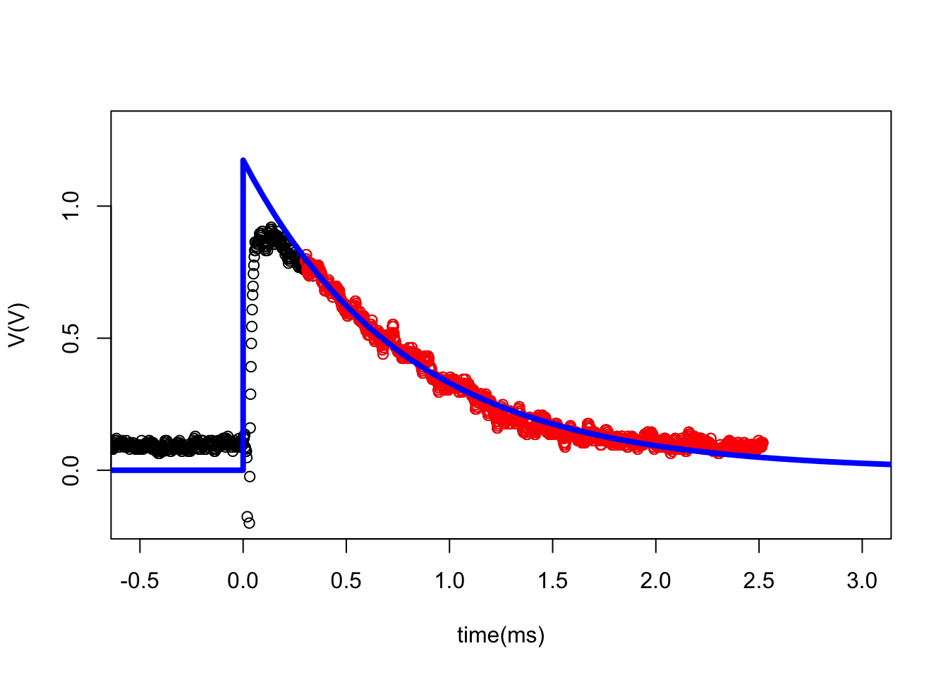
provides a straight-forward way to make a non-linear fit to the data
using the command nls, which takes 3 main parameters. The first
parameter is the data frame that contains the data to be fit. Next the
model is described, which is \(V = A \exp [ - time / T ]\), where \(A\) and
\(T\) are fitting parameters, and the others are variables defined in the
data frame. The fit will only work, if reasonable starting fit
parameters are provided. The starting parameters are provided in the
form of a list. The result of the fit is stored in a variable called
fit.
Measurement of a free induction decay from protons in glycerin. The graph is generated with R, where data points (circle) represent voltage measured after a 90\(^o\) pulse was applied to create precession. The relaxation of the signal amplitude is modeled and fit with an exponential decay.
The fit line is added to the plot by using predict to compute values
along some time values. In this case a vector with 100 elements is
generated, the time running from 0 to two times the maximum. The fit is
overlaid using blue color and line thickness of 4. The result of this
code is shown in Fig. 1.4.
library(ggplot2)
myData = data.frame(time = time.ms.fit, V = V.fit)
myData = rbind(myData, cbind(time = data$time.ms, V = data$V.V))
myData$label = c(rep("fit",length(time.ms.fit)),
rep("data", nrow(data)))
ggplot(myData, aes(time, V, color=label, linetype= label))+
  geom_point(size=1, alpha=0.8) + theme_bw(base_size=22) +
  xlab("time (s)") + ylab("V (V)") +
  scale_y_continuous(limits=c(-0.2,1.4)) +
  scale_x_continuous(limits=c(-0.8, 2.6),
  breaks=seq(-0.5,2.5,0.5)) +
  theme(legend.position = c(0.1, 0.9),
  legend.title = element_text(color=NA),
  legend.key = element_rect(colour = NA))
## Warning: Removed 893 rows containing missing values (geom_point).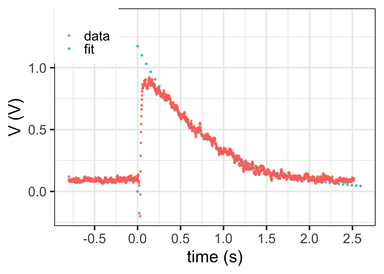
It is noteworthy that plot will clear the graph, but you can still add
data later using either lines or points for adding data with a line
or data points, respectively. The fitting parameters can be separately
listed with summary(fit)$coeff.
The same plot can also be graphed with the previously mentioned
ggplot2 package. A common way to use ggplot is to make a table with
three columns (using melt package for complex data). The first column
is the x-axis, the second the y-axis, and the third column defines the
data set for which automatically a legend is displayed. In the following
example, the NMR data is appended to the fitting data, by using the row
binding function rbind. The third column is called label and is
filled with the label for each row. The command length returns the
number of items in a vector and nrow returns the number of rows of a
data frame. Finally, the axes are labeled and the title of the legend,
which would be "label", is hidden. The legend.key element defines
the square around each of the items in the legend.