Chapter 10 Experiment: AFM
I lost all respect for angstroms. - Heinrich Rohrer
Atomic force microscopy is a common instrument in many science laboratories to go beyond the limitations of the optical microscope. Nanotechnology is invariably linked with measurements and analysis of features below the micrometer limit.
10.1 Exp I: Calibration Sample
We will use the EasyScan 2 AFM from Nanosurf to take AFM images. This device can measure the topography of a sample at nanometer resolution.
The EasyScan 2 AFM comes with a detailed manual explaining the operation. It requires three components. A computer for data acquisition, which is connected via a USB cable to the controller module. The controller module uses the Scan Head cable connector to connect with the scan head, a very delicate instrument. The Scan Head is placed on top of the stage using a tripod. The legs’ length of the tripod is changed via screws.
Note: never touch the cantilever tips or any part of the cantilever deflection detection system. The cantilever should be approached to the surface with great care. After finishing the scan, the scan head must be raised sufficiently before the sample can be moved out. The Scan Head uses a laser to measure the cantilever deflection, therefore when turning the Scan Head around, make sure to always place the DropStop at the end.
Note: the Scan Head should always have a cantilever installed, otherwise the spring may damage the alignment chip.
After installing the system, inspect whether the cantilever is properly installed. Use either viewport on the Scan Head to inspect the cantilever.
10.2 Turning on the easyScan AFM
The software program is already installed on the computer. After connecting the controller to the mains power, switch the controller on and watch the lights on top of the controller to light up. Wait a few seconds for the process to complete. Next, start the controller software on the computer. A window will pop up and it will now communicate with the controller to initialize the components. During this process, monitor the lights on the controller. All the detected components will light up. If no scan head is detected, the lights will blink.
Choose the dynamic force operating mode. In order to find the resonance frequency, indicate that the cantilever is similar to “ACL-A”. In general, you will be using an Aspire cantilever, which has a typical resonance frequency in the range of 160 – 180 kHz.
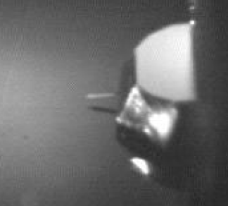
The reflection of the cantilever indicates that the cantilever is very close to the surface. Coarse approach is finished at this point.
10.3 Mounting Samples
Since there is sample drift, especially for small images, the sample needs to be mounted well. The sample holder is magnetic and can easily slide on the sample stage. Use a double-sticky tape to create a sticky area in the middle of the sample holder. On top of the double-sticky tape, add the post-it note. The sticky part should be up, so that the post-it note is secured with the double-sticky tape. Press down and make sure you have a firm and flat surface. The sample can then be mounted on top of the slightly sticky post-it note. Ensure that the post-it note area is larger than the sample area.
Add the sample using tweezers, then slide it over the stage under the cantilever. Take extra care that the Scan Head is high enough so that the cantilever has enough clearance above the sample after insertion. Use the three screws on the tripod Scan Head to lower the sample into proximity. At first use, eye the approach. Once you get close enough, look through the view port and identify the reflection of the cantilever on the surface. As you lower the sample further, the reflection and cantilever get closer as shown in Fig.~\(\ref{fig:cantileverOptical}\). This is referred to as the coarse approach.
10.4 Measurement
For the measurement scan, the sample needs to be very close to the surface. Typical distances are a few nanometers from the surface for dynamic mode. After coarse approach (see Fig.~\(\ref{fig:cantileverOptical}\)), use the following sequence to start imaging:
- Acquisition \(\rightarrow\) Frequency Sweep \(\rightarrow\) Auto Set
- Capture the Fine Sweep (range of about 2 kHz) for calculating Q-value
- Click on “Approach”, the green light should be on, “Approach Done” message appears
- Click on “Start” after setting parameters for image size, etc.
- Click on “Stop” to interrupt the measurement, and readjust parameters, or “Finish” for the last image
The finished images are automatically stored (although you can take additional images with the “Capture” button) until the program quits. Go to the “Gallery” to view the images and permanently store them on the disk. Make sure to use proper naming conditions.
The lights on the controller can be either red, orange, or green. If the light is red, it indicates that the scanner is in the upper limit position. In other words, the sample is too close to the tip. On the other hand, if the orange (yellow) light is on, it means that the sacnner is in the lower limit position. The sample-tip interaction is weak or the tip is too far away from the sample. It could also mean that the tip is not tuned, or the resonance curve does not show strong peaks; i.e. the tip is bad. The green light indicates normal operation. If the green light is blinking, then the feedback loop in the software has been turned off.
10.5 Improving Image Quality
The image quality will depend on the parameters that you choose. At the basic level, you choose the size of the image (Image size), the resolution (points / line), and the scanning speed (time / line). You can also select the scanning direction. Since there is a fast and slow scan axis in rastering and image, it is important to ensure that the fast-scan axis is not sloped. Invariably, at the nanometer scale, the sample will not appear flat, and you need to determine a good scanning direction by changing the rotation angle. If you have a step edge, it is advantageous, if the fast axis is perpendicular to the step edge.
In the *Advanced Level}, the z-controller’s integral and proportional gain can be controlled. Depending on the size and speed, these gains need to be adjusted. See the discussion on PID in Sec.@(adjustments).
10.6 Turning Off
Before finishing, you should make sure that all measurements have been saved. Be very attentive not to damage the tip as it is so close to the surface.
- Stop or Finish the image capturing
- Save all images
- Click on “Retract”, which watching the cantilever rise in the viewport
- Use the tripod to carefully and slowly raise the cantilever to a save distance
- Remove the sample carefully and without damaging the tip
- Exit NanoSurf Control software
- Turn off power to controller
- remove the cable from the Scan Head
- remove the USB cable
- carefully store the controller and Scan Head in the suitcase
10.7 Adjustments
The image can be improved using several methods. The first method is to change the rotating angle. You can attempt to make the plane level during the scan. Additionally, you can adjust the PID parameters.
Due to the scan speed and the variation in topography, it is important to control the cantilever height precisely. However, different sample topographies require adjustments in the “reaction” speed of the cantilever. Therefore, there will be an error signal, which is defined as the difference between the cantilever height and the actual object’s height. Naturally, faster scans are prone to increase the error signal. If you scan forward and backwards on the same line, the error may become very visible.
In order to minimize the error signal, it can adjusted with the proportional - integral - derivative (PID) parameters, see Sec.~\(\ref{sec:PID}\). These three parameters should be set in this order: proportion, integration, differential. Increasing the P-gain will decrease the error signal, whereas increasing the I-gain will decrease the error signal over time. The differential parameter is difficult to set accurately as it is proportional to the derivative of the error signal. All three parameters are explained in Fig.~\(\ref{fig:PID}\).
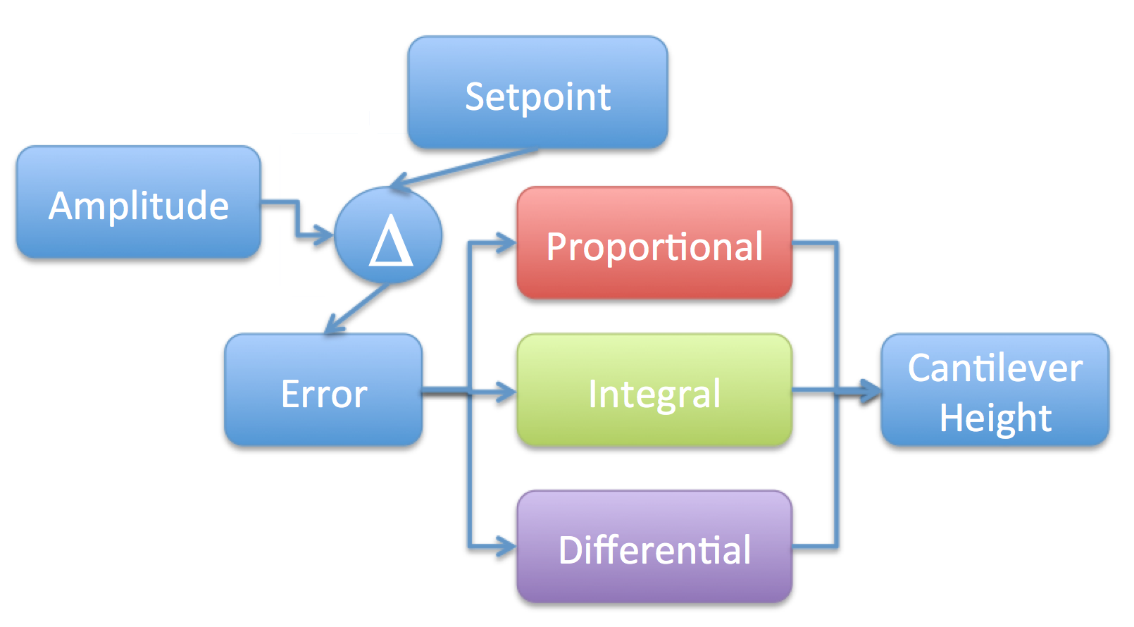
The difference between the amplitude and the setpoint is computed and regarded as the error signal. It is then processed through the PID and summed to adjust the piezo for the z position.
For good AFM results a vibration isolation platform is necessary. The vibration isolation consists of a large mass attached to springs. Between the low resonance frequency of the isolation system and the high resonance frequency of the microscope hardware itself (> 10 kHz), the AFM effectively comprises a band pass filter. This allows the user to safely image their samples in the intermediate range of about 1 – 100 Hz and obtain good resolution.
10.8 Exp II: Data Storage Sample
On storage media, such as CD and DVDs, the data is written by indentation into a polycarbonate surface. The pits can be imaged with the AFM and several parameters related to the storage technology can be extracted, see Table~@(tab:storage-media). This includes the pit depth, width, pit separation, and pit length. Use the results from the calibration sample to determine all four parameters for the sample provided. A laser beam is scanned across the surface and the reflection of a pit or surface is measured with a photo-diode at a rate of \(\sim\) 1 MB/s for a DVD.
Data on a CD is generally encoded with eight-to-fourteen modulation (EFM). In essence, one byte, which corresponds to 8 bits, is stored as a 14-bit pattern. Therefore, a series with 14 zeros and ones corresponds to 1 byte of data. The additional 6 bits are used to make the data error-free and provide tolerance, if the reader is going a bit faster or slower, or could not read a bit correctly.
%To understand the difference between a CD and DVD, let’s look at the details. (Show slide 2.) CDs and DVDs store large amounts of binary data (those patterns of 0s and 1s), which a CD/DVD player can read using a laser, optical devices and sophisticated electronics. CDs and DVDs are made mostly of plastic (polycarbonate) and can store more information by having multiple recording layers. The data is stored in a series of tiny pits, arranged in a spiral, tracking from the center of the disk to the edge. (Show slide 3.) The data layer is coated with a thin layer of aluminum or silver, making it highly reflective. If stretched out, this spiral of pits would be about 5 km long! The pit length and the distance between pits define the digital data. The depth of a pit is 0.11 ?m and the width is 0.5 ?m. Its length varies between 0.83 and 3.56 ?m.
| Media | Year | Size (GB) | Laser(nm) | Diameter (nm) |
|---|---|---|---|---|
| Vinyl Record | 305 | |||
| CD | 1983 | 0.7 | 780 | 120 |
| DVD | 1996 | 4 – 8 | 650 | |
| Blu-Ray | 2006 | 25 – 50 | 405 | 120 |
| BD-XL | 2010 | 128 | 405 | 120 |
As a interesting separate experiment, you could determine the storage capacity by shining a laser beam of known wavelength at the CD, DVD or other storage media and from the diffraction pattern determine the storage density.
10.9 Image Processing
The atomic force microscopy (AFM) images are stored in different formats depending on the AFM vendor. Generally, these files include a header section that contains information about how the image was recorded, such as the tip’s set point, scanning size, maximum height, PID parameters. This section is followed by height information for each pixel of the image. Generally, the height is limited to a resolution of 8 bits.
There are several programs available for Image analysis. The most commonly and freely available programs for download are:
- R package: nanoscopeAFM
- WSxM (Horcas et al. 2007)
- Gwyddion (Klapetek, Necas, and Anderson 2016)
- Image SXM
- n-Surf Image
- ImageJ for image processing, but cannot open AFM images directly
Once the image is loaded, the first step is generally to flatten the image. Since the image contains “raw” data corresponding to the piezosensor’s output voltage, the sample surface is often not flat with respect to the head. Different algorithms exist to subtract the background, the most common being a “plane level” method. It uses all data points and computes a common plane level that can be subtracted. If there are a streaks in the image that were caused by a bouncing cantilever, they can also be removed.
The processed image can now be evaluated to extract different quantities, the following quantities are most relevant:
- surface rms roughness
- minimum and maximum height
- height bin distribution and symmetry
- mean height, average height
- autocorrelation length (Klapetek, Necas, and Anderson 2016)
- average grain size
- height-height correlation length
- power spectral density function
- wavelet transform
The AFM is a powerful tool to measure the surface roughness; however due to the coupling of tip and surface care must be taken in the data’s interpretation. Experimentally, Sedin and Rowlen demonstrated that there might be two different trends for measured surface roughness as a function of tip size as found in stylus measurements (Sedin and Rowlen 2001). They showed that at small lateral scan sizes the image RMS roughness decreased as tip size increased. However, at larger scan sizes (\(>5 \mu\)m) the roughness increased with increasing tip size.
It is widely known that most significant features of a random surface can be completely defined by two parameters: the height distribution and the correlation distance (Chen and Huang 2004). For AFM measurements, we usually evaluate the one-dimensional autocorrelation function based only on profiles along the fast scanning axis. It can therefore be evaluated from discrete AFM data values using this transform:
\[\begin{equation} G_x(\tau_x)=\sigma^2 \exp \left( \frac{-\tau_x^2}{\xi^2} \right) \end{equation}\]
where \(\sigma\) denotes the root mean square (rms) deviation of the heights and \(\xi\) denotes the autocorrelation length.
The difference between the *height-height correlation} function and the autocorrelation function is very small. As with the autocorrelation function, we sum the multiplication of two different values. For the autocorrelation function, these values represented the different distances between points. For the height-height correlation function, we instead use the power of difference between the points.
The height difference correlation function (HDCF) is measured as follows,(Gredig, Silverstein, and Byrne 2013)
\[\begin{equation} g(|\vec{r}|) = <\left( h(\vec{d})-h(\vec{d}+\vec{r}) \right)^2>, \end{equation}\]
where \(h(\vec{d})\) is the height of the sample at position \(\vec{d}\). The 1D height-height correlation function is often assumed to be Gaussian and can be expressed in this expression of Hurst,
\[\begin{equation} g(r) = 2\sigma^2(1-\exp\left( -r/\xi \right)^{2H}), \end{equation}\] where \(\sigma\) is the long-range roughness for \(r>\xi\), \(H\) the short-range roughness and \(\xi\) the correlation length. The Hurst parameter \(H\) is generally a number from 0.5 to 1.0 and describes the fractal dimension of the surface, where \(D=3-H\) (Mandelbrot 1983). The correlation length is directly proportional to the average grain size, usually by a factor of 2 to 3 (Gredig, Silverstein, and Byrne 2013). Thus, the correlation function provides an easy measure of the average grain size.
The grain size can be further investigated using a Watershed algorithm (Gentry, Gredig, and Schuller 2009). This algorithm is implemented in the ImageJ software and can be used to create exact grain size distributions.
10.11 AFM Lab Report
The AFM lab report includes an image of the calibration sample and analyzes the height and width using line profiles. In the second part, an image of the storage device is shown. Discuss the data density that you obtain from the AFM images. You may also discuss how the shape of the trenches that you found, and provide a histogram of the lengths.
10.12 Predictions
Small nano-spheres of 50 nm diameter are randomly deposited on a perfectly flat substrate. Discuss various possibilities of what you observe with an AFM tip depending on the density of spheres. Assume that the tip has a curvature of 20 nm and is otherwise shaped like a pyramid. Draw a line trace that shows the spheres and the AFM tip as it traces the surface.
PID parameters are often used to control the temperature, say an oven uses a PID controller to set the temperature above room temperature. Draw what happens to the temperature as a function of time for a large (mass) oven with a small heater that has both I and D set to 0 and only uses P.
What are autocorrelation functions? How is the autocorrelation length computed? What is the meaning of the autocorrelation length?
Calculate the total length of pits on a typical DVD.
Estimate the amount of data you could store on a vinyl record disk using digital encoding.