Chapter 9 Experiment: NMR
I am sure my fellow-scientists will agree with me if I say that whatever we were able to achieve in our later years had its origin in the experiences of our youth and in the hopes and wishes which were formed before and during our time as students. – Felix Bloch
The background for pulsed nuclear magnetic resonance (NMR) is detailed in section @ref(nuclear-magnetic-resonance}. It is a testament of ingenuity in science that it is possible to easily probe the spin of a nucleus deep inside an atom. The experiment is based on pulsed and continuous wave nuclear magnetic resonance apparatus from TeachSpin. It has a magnet that provides a strong and constant magnet field to polarize spins of protons. The pulse generator can create a sequence of short RF pulses for adding a torque finely tuned to the nuclear spin. The signal is read out with the receiver coils and then amplified to be viewed on an . Given this setup, it is possible to determine the spin-lattice relaxation time and the spin-spin relaxation time of glycerol (C\(_3\)H\(_5\)(OH)\(_3\)) and other proton-rich viscous liquids. Secondly, you can determine the homogeneity of the magnetic field to high accuracy using the frequency of the protons. Finally, analysis and Fourier transform of the RF signal shows you frequency spectrum.
After carefully reading the TeachSpin manual, create a number of pulse sequences and view them with the (see section @ref(oscilloscope}. Next, prepare a sample with glycerine or another viscous liquid, connect the pulse generator, amplifier, and detector using BNC cables, and then tune to the resonance frequency of the protons. The resonance frequency will vary every day as the magnetic field changes slightly with temperature in the room. After finding the resonance frequency, make a measurement of the free induction decay, all the time making sure that you optimize the position of the sample. At this moment, you can find the spin-lattice relaxation, at first using an estimation, and then by varying the delay time between the two pulses. The last part of the experiment will be the measurement of the spin-spin relaxation time. If time and interest allow, carefully map the magnetic field in the sample plane and determine inhomogeneities. In the following, details are provided to make these measurements. Keep in mind that it is important to understand the background from section @ref(nuclear-magnetic-resonance} in order to follow the abbreviated steps. No attempt is made to provide a detailed and complete description of the steps necessary to complete these measurements, as the experiment should be completed in an exploratory fashion for optimal learning outcomes.
Goals for this section:
Create Standard Operation Procedure ()
Operate to view pulse sequences
Measure the (FID) signal
Measure the inhomogeneity of the magnetic field using the resonance frequency mapping technique
Determine \(T_1\) in a glycerine sample
Determine \(T_2\) in a glycerine sample using Meiboom-Gill sequence
Write a Single-spaced 3-6 paged report
9.1 Oscilloscope
The allows you to track very fast signals precisely. The Tektronix TDS 2002 has two or four input channels that can be displayed all at once or separately. You may be using a different model, so make sure to note the bandwidth and the sample rate. After powering on, you will need to wait a few seconds for the to boot, it will resume the configuration it had, when it was last used. The manual for the can be downloaded and is available online, familiarize yourself with the functionality of the tool before using it.
The shows time along the x-axis and voltage on the y-axis. The time dependent voltage signal is fed through the BNC connectors to one of the channels. Often short pulses that last on the order of 10 μs need to be measured and cannot be resolved in real-time. Therefore, the has an external , which is a separate input channel. The trigger signal - sometimes also referred to as the synchronization signal - is generally a single short peak sent out at the time of interest. The display will then hold a short window centered around the trigger signal until the next trigger signal arrives. Depending on the trigger signal, the threshold or trigger level is adjusted to avoid false triggering. A good starting point to set the trigger properly is to use the "Set to 50%" button, which determines the maximum voltage signal from the trigger and then sets the level to the half point as the maximum voltage. The trigger signal will fluctuate a little bit.
The "Holdoff" can be used to set the amount of time before another trigger event is accepted; this can substantially improve flickering of the signal.
Data from the is stored using an external USB drive, which is automatically recognized once connected. Pressing the "save data" button will allow you to save three files, the settings of the , a capture of the screen image, and most useful, the data points of all the channels which are turned on. At this point, it is important to write down the filename in the lab notebook.
For each channel, the TDS 2002 will store 2500 points. That means, if you set the to capture a screen with 100 μs, each data point is separated by 40 ns, if the recording is at a rate of 25 MHz. The estimate becomes important, when you are performing a Fourier transform of an oscillating signal as it defines the resolution necessary for resolving a particular signal. In the sample given, frequencies in the range from 2.5 MHz to roughly 0.1 MHz can be resolved. The CSV file should be used for generating graphs. A method is described in section ??.
Use the "measure" button to obtain data directly from the display. Use the "average" functionality to average over several signals. The "Single Seq" button acquires a single sequence and then stops measuring. There are many other useful signal processing events built into the . You can vastly increase the accuracy of your measurement by understanding the full functionality capability of the oscilloscope.
9.2 NMR Instrumentation Basics
A permanent magnet creates the strong magnetic field in the z-direction. In our experiment the z-direction is parallel to the table. The sample in the test tube can be moved in all three dimensions by using two separate adjustments. The planar position is controlled with two knobs from the yz-stage, which can be carefully rotated. The third dimension is adjusted with the o-ring attached to the glass tube with the glycerine. The magnitude of this magnetic field can be measured by tuning to the resonance frequency at each location. Since the frequency is directly related to the magnetic field strength, the resulting map provides insight into the inhomogeneities of the permanent magnet.
The second magnetic field is much smaller in magnitude. Therefore, a small coil produces the magnetic field pulse using the . You can measure the magnitude of this secondary magnetic field using a test tube with a pickup coil inside. Using the geometry of the pick-up coil and an , you can determine the magnitude of this field. The sample will then RF radiate and this excitation is measured with a secondary RF coil through Faraday induction. The following components are used, find out where each of the following components are located and draw a diagram of how they are connected in your lab notebook.
permanent magnet
pulse generator
RF oscillator
pulse amplifier
receiver
linear detector
A block diagram of the TeachSpin apparatus is shown in Fig. ??. A permanent magnet supplies the field \(\vec{B}_0\) along the z-axis (which in this instrument is not vertical but parallel to the table). The rotating magnetic field \(\vec{B}_1\) is supplied by a Helmholtz coil with its axis perpendicular to the axis of the sample test tube. The field this coil supplies, of course, is actually linear, not rotating, but any linearly polarized field can be thought of as the sum of two counter-rotating fields. In our case only the component that matters is the one rotating along with the precessing spins. The other one can be neglected.
The magnetization produced by the sample does rotate, and because of this the receiver coil, labeled "probe" in Fig.??, can be oriented perpendicular to the Helmholtz coil.
Block diagram of the pulsed-NMR apparatus used in this lab. In this setup, an RF synthesized oscillator is gated by a pulse programmer to produce, through an RF amplifier, an oscillating magnetic field \(\vec{B}_1\) in the sample. Note carefully the orientation of the coils around the sample! As shown in this figure, the permanent magnetic field is applied perpendicular to the page; the applied magnetic field B is orthogonal to the axis of the sample tube; and the axis of the receiver coils is parallel to the test tube’s axis. The output of the receiver goes both to a mixer (analog multiplier) and to tan RF amplitude detector (rectifier), and the outputs of these are displayed on an .
Read 2.TeachSpinNMR Instrument.pdf for the individual components. You may want to have the file available while you are doing the experiment.
In particular, follow the precautions on p. 21 of the TeachSpin manual.
Please be extremely careful with the magnet, as described in the TeachSpin manual. Do not drop or shake the magnet, do not bring magnetic objects near the magnet, and do not drop magnetic objects in the sample probe. Do not force the sample probe past its limits of travel.
Do not operate the power amplifier without attaching the TNC cable2 from the sample probe.
Do not operate the pulsed NMR unit with pulse larger than 1%. Duty cycles over 1% will cause overheating of the output power transistors.
9.3 Prediction
Turn in the following predictions before starting the experiment.
Show a diagram of all major components of the TeachSpin NMR instrumentations and show how the cables are connected.
Make a graph of a typical free induction decay, where you plot the voltage versus time.
Show how you can extract the approximate time of \(T_1\). Provide a step-by-step instruction set.
9.4 Exp I: Lattice-Spin Relaxation
9.4.1 Pulse Programming
Follow the step-by-step instructions in 3. TeachSpinNMR GettingStarted.pdf in order to create several pulse sequences.
First, generate a single pulse. Set the time to 1.0 ms/cm and the repetition time to 10 ms and change the variable repetition time from 10% to 100%. What do you observe? Write down your observation in your lab notebook.
The programmer has two pulses which it can generate. The second pulse can be repeated up to 99 times. Change the A and B width, change delay time, change sync to B, turn A off, change repetition time, and observe what happens. Look at a two pulse train with delay times from 1 to 100 ms. Pick one condition and sketch what you observe in your lab notebook. Don’t forget to make note of the delay time, repetition time, and what signal you are triggering from. Also view the trigger pulse. How long is the triggering pulse?
Follow the instructions in "3. TeachSpinNMR GettingStarted.pdf" to generate several pulses of different widths.
9.4.2 Receiver Calibration
Supplied with the instrument are two vials with small loops of wire embedded in epoxy and coaxial cables connected to these loops. Notice that the two coils have different orientations. One is designed for measuring B, and the other is designed for generating a false signal in the pickup coil.
Read this section about tuning the receiver. You will need to tune the receiver to the oscillator frequency using a special dummy signal probe. Choose the appropriate coil configuration to do this measurement. Explain the rationale of your choice. Sketch the trace in your notebook when the receiver is tuned.
9.4.3 Measurement of the Permanent Magnetic Field
The first experiment we are going to do is look at the applied magnetic field B of the permanent magnet. Supplied with the instrument are two vials with small loops of wire embedded in epoxy and coaxial cables connected to these loops. We will observe B and measure its amplitude by placing one of these coils in the sample space and looking at the voltage induced by the oscillating B field.
Notice that the two coils have different orientations. One coil is designed for measuring B, and the other is designed for generating a false signal in the pickup coil. For the orientation of RF generating coil refer to Fig.??. Which coil should you use to measure B and what is the orientation? What is the relationship between the voltage generated across the coil and B? What property of the coil do you need to measure to convert between this voltage and B? (This will just be a rough estimate, so don’t spend too much time on precision here. An error of $$20% will be fine.) Clearly describe your procedure for measuring B in your lab notebook, along with the formula you use for converting your observed voltage to B and how you arrived at it.
If there are any cables connected to the front panel of the TeachSpin electronics bin, disconnect them and turn the instrument on. (The switch is in the back.) Locate the A+B OUT port, in the PULSE PROGRAMMER module. Using a tee, connect this to the A+B IN port on the 15 MHz OSC/AMP/MIXER module and then to the other channel of your . Trigger the scope off of the SYNC OUT signal, provided by the pulse programmer module. The blue cable attached to the sample holder with the TNC connector (see footnote on page ) on the end of it supplies current to the Helmholtz coil. Plug this into the RF OUT port on the 15 MHz OSC/AMP/MIXER module. Also connect the BNC end of the coil you placed in the sample space to Ch 2 of your .
Because this instrument is designed for pulsed NMR, the RF oscillator is gated by the pulse programmer. When the voltage going into the A+B IN port is high, a signal is applied to the coils. When it is low (zero), no current flows through the coils, and no magnetic field is applied. The length of time over which the field is applied is set by the A-WIDTH knob on the pulse programmer module. On the pulse programmer module, make sure that MODE is set to INT, the SYNC switch is set to A, the A switch is ON, and the B switch is OFF.
You should now see both the gating signal (from Scope Ch1 ) and an RF signal (Scope Ch2) on your screen. Make sure your coil is optimally aligned, measure the amplitude of the RF signal you observe, and use this to estimate the magnitude of B. Estimate how long this signal should be applied to produce a pulse. Sketch the traces in your notebook and include it in your lab notebook.
When you are done this part, remove the test coil from the sample space and disconnect it from your .
9.4.4 Larmor Frequency
The magnetic field strength of the magnet depends on the room temperature and sample location. Therefore, the precise frequency must be tuned every time and may need to be readjusted every half hour. involves the observation of beating on the oscilloscope. The beating pattern is generated by mixing two frequencies which are similar. The first signal is from the RF generator, which is mixed, see Fig.??, with the receiving signal from the sample.
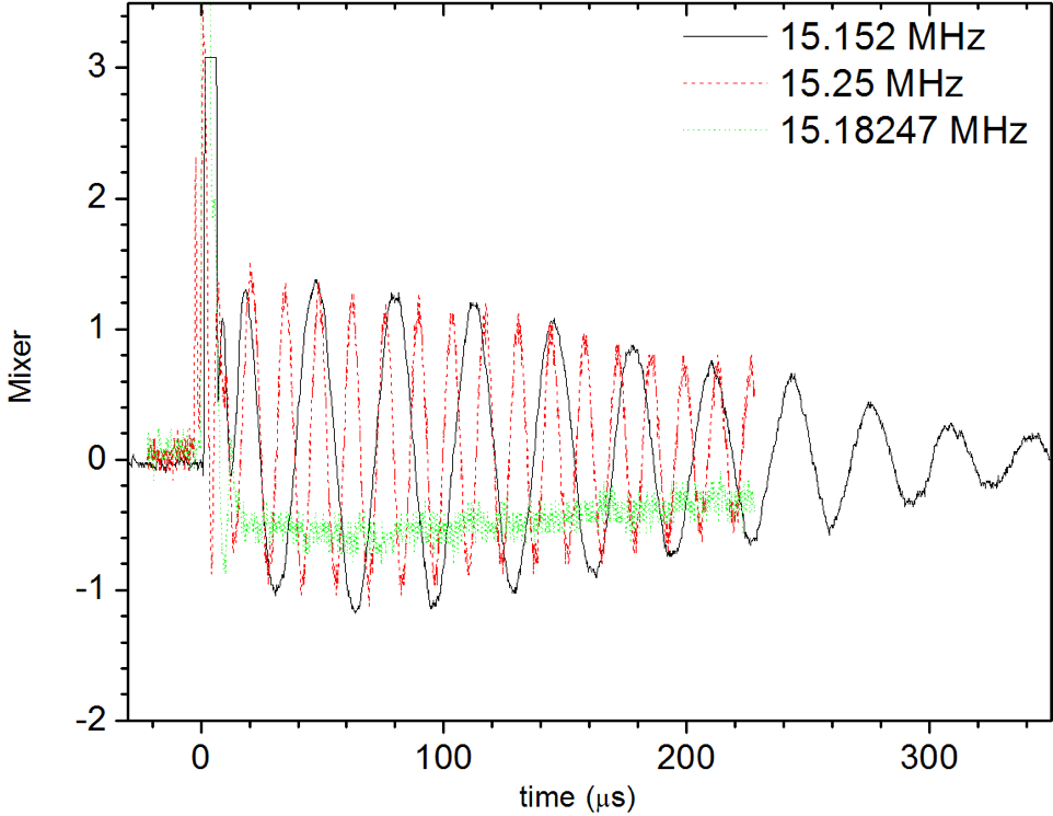
Beating patters are observed on the oscilloscope, when the RF coil’s frequency does not match the Larmor frequency. Beating is observed both at 15.152 MHz and at 15.25 MHz. However, the beating is minimized at 15.18247 MHz, which means that the provided RF generator frequency is the same as the Larmor frequency from the sample.
9.4.5 Free Induction Decay Experiment
FID (Free Induction Decay or Free Precession Decay) Use Glycerin sample for this part of experiment. Glycerin and mineral oil have similar T\(_1\).
1. You have already done the first option in the beginning of the experiment. Skip this part.
2. Follow the setup. It is extremely important to find the zero condition. Turn on CW-RF (CW-RF switch must be off after finding the zero beat condition). If the oscillator is properly tuned to the resonance, the MIXER OUT shows no beat. If the MIXER OUT (Ch2 in the ) looks like the beating pattern in Fig. ??, then the oscillator is not properly tuned. Adjust the frequency using FREQUENCY ADJUST knob in the 15 MHz RECEIVER module while monitoring the MIXER OUT signal. The zero beat condition is when there is no beating from the MIXER OUT and two traces in the are as close as possible. Sketch the trace of the MIXER OUT and write down the zero beat condition frequency. You can find a bit more information about this process in 2. TeachSpinNMR Instrument.pdf.
After finding the zero beat condition, turn on CW-RF switch. Turn the A-WIDTH knob and monitor Ch1 (DETECTOR OUT). The shortest A-width pulse that produces the maximum amplitude of FID is pulse. Sketch the trace of the DETECTOR OUT with pulse, record the maximum amplitude, and measure the A-width.
Follow the instructions in the manual. You should be familiar with all the procedures in this part already. Measure the magnetic field in at least 3 x 3 points by changing x- and y-positions. Record the resonance frequency in the lab notebook. Show the calculation for the magnetic field. Use to produce the surface plot of magnetic fields in xy-plane.
9.4.6 Spin Lattice Relaxation Time, T\(_1\)
Our goal is to obtain T\(_1\) from Glycerin. Your group needs to produce a standard operating procedure on how to measure T\(_1\). 5.TeachSpinNMR Conept Tour.pdf has useful information, so you should read that. Sketch one typical trace. Record your raw data in the . Explain clearly what you should plot in x- and y-axis to obtain T\(_1\). Obtain T\(_1\). What is your error?
9.5 Exp II: Spin Echo and \(T_2\)
Our goal is to obtain T\(_2\) from . Your group needs to produce a standard operating procedure on how to measure T\(_2\). 5.TeachSpinNMR Concept Tour.pdf has useful information, so you should read that. Sketch one typical trace. Record your raw data in the lab notebook. Explain clearly what you should plot in \(x-\) and \(y-\)axis to obtain T\(_2\). Obtain T\(_2\). What is your error?
9.6 NMR Lab Report
The lab report should contain several important results and features. Therefore, make sure the following items have been recorded properly. For one, you should have a free induction decay graph. It may be useful to also record the pulse sequence. Secondly, for the measurement of the spin-lattice relaxation time \(T_1\), it is important to make measurements in correct intervals. The \(T_1\) value should be extracted using a fitting procedure.
A TNC (threaded Neill-Concelman) connector is similar to a BNC (Bayonet Neill-Concelman) connector, but instead of a twist it has a thread that is screwed in. The TNC is superior in performance at microwave frequencies.\[TNC\]↩︎