Chapter 6 Nuclear Magnetic Resonance
Many modern applications in physics, chemistry, biology, engineering, and medicine are based on the nuclear magnetic resonance (NMR) technique. We should recognize the enormous versatility of magnetic resonance and its successes not precluded to science, mathematics, and medicine. It is also an example of the service of physics towards other fields. Originally discovered in physics, it became an analytical tool in chemistry, and later an indispensible tool in medicine. For example, the relaxation time can be used to observe malignant tissues.(Damadian 1971) Despite almost a 100 years of research, new applications are still emerging. From a physics perspective, it makes sense to start with the most fundamental aspects of NMR, so this part will familiarize you with the pulsed nuclear magnetic resosnance (PNMR) method and its many applications. The part of NMR that makes it particularly useful are the determination of the spin-spin coupling, and also the chemical shifts from the electron shielded nuclei.
Related techniques include magnetic resonance imaging (MRI) and electron paramagnetic resonance (EPR), also known as electron spin resonance (ESR). This methods can also be understood after we have covered the fundamental pricniples of PNMR. Herein, we will use the 15 MHz PNMR setup, which allows for measurements of the free induction decay (FID) in glycerin (C3H8O3) and other proton-rich materials.
The phenomenon of NMR concerns the nucleus of an atom. Nuclear magnetic resonance spectra can be used to learn about how complex molecules are organized. The molecule is put in a constant magnetic field to generate an equilibrium spin distribution. Then, a magnetic pulse perturbs the system, such that nuclear spins (protons, neutrons) are excited and resonate between discrete energy levels. The emitted signal, (FID), can be picked up by coils and interpreted. The FID signal contains information about the chemistry of the atomic arrangement in the molecule. In magnetic resonance imaging (MRI), additionally a magnetic gradient is applied, the signal contains information about the density of nuclear spins in space and we can identify soft tissues.
The discovery of nuclear magnetic resonance (NMR) received several Nobel prizes, see Table 1.1. Additionally, other Nobel prizes were given to connected fields, such as the work for K.A. Müller on EPR.(Boesch 2004)
6.1 Nuclear Spin
As a natural consequence of the relativistic quantum mechanical Dirac equation from 1928, the notion of the spin has emerged. It describes not only the spin of the electron, but of other massive fermions with spin half, such as quarks. The nucleus (proton, neutron) also has a spin (I=1/2). All spins have quantized energies in multiples of \(\hbar\) and by extension an intrinsic angular momentum and magnetic momentum. Fundamentally, a magnetic field is produced by a moving charge.
These quanta are generally expressed in \(S\), \(L\) (angular momentum quantum number), and \(I\). The nucleus can have a spin (nuclear spin), which is generally denoted by \(I\). A free proton or neutron has a nuclear spin \(I=\frac{1}{2}\). Atoms can have more complex nuclear spins; it depends on the number of protons and neutrons. For even number of both protons and neutrons, I=0; but for an even number of one and odd number of the other, it has a half-integer spin. In the case that both are odd numbered, we have an integer spin. Examples include 12C, 16O with \(I=0\), 1H, 13C and 19F with \(I=1/2\), 11B with \(I=3/2\), 17O with \(I=5/2\), and 2H, 14N with \(I=1\).
The most important group is possibly the spin-\(\frac{1}{2}\) nuclides groups, which includes 24 elements or 31 isotopes that are non-radioactive. The useful elements are H,He, C, N, F, Si, P, Fe, Se, Y, Rh, Ag, Cd, Sn, Te, Xe, Tm, Yb, W, Os, Pt, Hg, Tl, and Pb. Amongst those, the most commonly used are 1H, 13C, 15N, 19F, and 31P.
Notably, the spin of the electron cannot be probed classically as pointed out by Bohr(Bohr 1925). It is a quantum-mechanical phenomenon. Charles G. Darwin, the grandson of the naturalist, led early investigations of the electron’s spin. Then, Wolfgang Pauli published a seminal paper on the exclusion principle in 1925. He deduced that nuclei should also possess an angular momentum (Pauli 1925) similar to electrons. Earlier, the experimental results from Paschen showed spectral lines that were not expected, but if one understood, as Goudsmit (student of Ehrenfest) and Uhlenbeck did, that the electron carries both an angular momentum and an intrinsic spin with their associated quantum numbers \(m_l\) and \(m_s\), then the spectrum could be explained. The electron spin, then, could also explain some complicated Zeeman effects and everything fell into place. The neutron in the nucleus had, of course, not been discovered yet. In 1932, Chadwick, student of Rutherford, published the possible existence of a neutron in an opinion piece called Letters to the Editor in Nature (Chadwick 1932) after trying to understand the ionisation mesurements of Nobel laureate Irène Joliot-Curie, daughter of Marie Curie. While it was at first clear that the electron had an intrinsic spin, it became understood that the proton and the neutron would also contain spin. While the electron’s angular momentum can be conceptualized classically (orbital motion), the nuclear’s spin cannot be perceived as such, as it is purely a quantum mechanical phenomenon. Even though protons have a complicated structure based on quarks and gluons, the spin is rather simple, just one half. It is estimated that about half of the proton’s spin originates from the gluons, while about a third comes from the three quarks, leaving some unknowns.
On the experimental side, Rabi took on the task to find the nuclear spin of sodium.(Rabi and Cohen 1934) His character was such that he wanted to design a simple, clean, and clever experiment to measure it. So, in 1937 Rabi predicted that by a radio-frequency excitation signal to the frequency, the absorbed energy could flip the spin orientation. A year later, his team succeeded in observing the magnetic resonance phenomenon that was specific or characteristic to each atom or molecule. While this work was focused on atoms, Ed Purcell (Harvard) and Felix Bloch (Stanford) extended the method to liquids and solids a few years later. Erwin Hahn observed that there is a spin echo in 1949 (Hahn 1950). (This experiment will be performed in Sec.9.5. At the same time, chemical shifts were observed due to the local changes in magnetic fields from electron cloud shielding inside molecules. In the medical field, NMR was first used in 1977 to generate a two-dimensional image of the proton density of soft tissues, what is now known as magnetic resonance imaging (MRI). This technique relies on mathematical Fourier transformations, which became more feasible with the growth in computational technologies. While NMR was initially developed in physics, it spread quickly into chemistry, bio-chemistry and medicine. With the advent of quantum computers, ideas based using NMR to build quantum computers are also explored.
| Year | Person | Title |
|---|---|---|
| 1943 | Otto Stern | development of molecular ray method and his discovery of the magnetic moment of the proton |
| 1944 | Isidor Isaac Rabi | resonance method for recording the magnetic properties of atomic nuclei |
| 1952 | Ed Purcell, Felix Bloch | development of new methods for nuclear magnetic precision measurements |
| 1991 | Richard Ernst | method of high-resolution NMR spectroscopy |
| 2002 | Kurt Wüthrich | using NMR for determining the three-dimensional structure of biological macromolecules |
| 2003 | P. Lauterbur, P. Mansfield | for discoveries concerning magnetic resosnance imaging |
6.2 Nuclear Magnetic Moment
Let us start on some common ground - for brevity’s reasons and without compromising the end result too much - from a classical perspective. For an electron on a classical orbit, the magnetic moment \(\mu\) is defined by its current density \(\vec{j}\):
\[ \vec{\mu} \equiv \frac{1}{2} \int \vec{r} \times \vec{j} \; d^3r, \]
which can be rewritten - for the purpose of clarity here - for a uniform current density with the current \(I\) and the cross-sectional area \(A = \pi R^2\) of a wire. It then follows that for a single electron that the magnetic moment is expressed as
\[ \mu = I A = \frac{e}{T} \pi R^2, \]
where \(T\) is the classical time that the electron takes to orbit the nucleus once. This time can be expressed as \(T = \frac{2\pi R}{v}\), such that orbital magnetic moment of the electron is
\[ \mu = \frac{e}{2}vR = \frac{e}{2m_e} L. \]
The classical angular momentum \(L\) is the product of \(m_e R v\). Quantum-mechanically, \(L\) is quantized, where \(L=N\hbar\) and N is an integer. It is then natural to define the smallest magnetic moment - called Bohr magneton - which is given by
\[ \mu_B = \frac{e \hbar}{2 m_e}, \]
where \(e\) is the charge of the electron and \(m_e\) the mass of the electron. Since the proton is quite a bit heavier, the magnetic moment from its spin is smaller by the same fraction.
Now, we can define the magnetic moment quite generally as:
\[\begin{equation} \mu = g_{I} \frac{e \hbar}{2 m_{e,p}} m_{I} \tag{6.1} \end{equation}\]
where \(g_I\) is the gyromagnetic factor, \(m_{e,p}\) is the mass of the electron or proton respectively, and \(m_{I}\) are the quantum numbers for electron spin, electron angular momentum and nuclear spin. For a proton \(m_I\) has only two values, namely \(\pm 1/2\).
It follows that due to the mass of the proton and neutron compared to the electron’s mass, the magnetic moment is about \(2000 \times\) smaller for nuclei. Therefore, electronic properties can largely ignore the nuclear spins.
The gyromagnetic factor takes into account the geometry of the particle. The value of g is \(g_S \simeq -2\), \(g_L = -1\), and \(g_I = 5.58\) for a proton and \(g_I = -3.82\) for a neutron. The discrepancy of the \(g_{I,p} / g_{I,n}\) ratio from 3/2 is due to the color charge of quarks explained in quantum chromodynamics.
The potential energy \(U\) of an atom with the nucleus spin aligned and anti-aligned to an external magnetic field \(\vec{B}\) is given by the following dot product.
\[ U = -\vec{\mu} \cdot \vec{B} \]
The energy difference for the hydrogen atom, which has only two states (between \(m_I=+1/2\) and \(m_I=-1/2\)), in a magnetic field along the z-direction \(B_z\) is
\[ \Delta E = g_I \frac{e \hbar}{2 m_p} B_z = \gamma \hbar B_z. \]
Here, the material specific property \(\gamma\) is called the gyromagnetic ratio and defined as,
\[\begin{equation} \gamma \equiv g_I \frac{e}{2 m_p} \tag{6.2} \end{equation}\]
| isotope | spin | magnetic | magnetogyric | NMR |
| \(I\) | moment | ratio \(\gamma\) | frequency | |
| electron | 0.5 | -3184.0 | -17610 | 65820.0 |
| neutron | 0.5 | -3.3 | -18 | 68.5 |
| hydrogen | 0.5 | 4.8 | 27 | 100.0 |
| \(^{13}\)C | 0.5 | 1.2 | 7 | 25.1 |
| \(^{19}\)F | 0.5 | 4.6 | 25 | 94.1 |
| \(^{23}\)Na | 1.5 | 2.9 | 7 | 26.5 |
| \(^{113}\)Cd | 0.5 | -1.1 | -6 | 22.2 |
| \(^{195}\)Pt | 0.5 | 1.0 | 6 | 21.4 |
Typical values for \(\gamma\) are listed in Tab. 1.2. The units of \(\gamma\) are energy per Tesla per Planck’s constant \(\hbar\). The energy gap \(\Delta E\) is directly proportional to the applied magnetic field with \(\gamma\) as the slope. The gap can be increased by increasing either the magnetic field or using nuclei with large \(\gamma\) values.
In an external magnetic field \(\vec{B}\) the nuclear spin will precess with an angular frequency \(\nu\), called the Larmor frequency. The precession is similar to the mechanical analogue of a bicycle tire precessing due to the force from the Earth. The precession becomes visible after an initial kick, see Fig. 1.1. Over time, the spinning bicycle wheel will relax back to its ground state with the angular spin aligned with the Earth’s gravitational field.
How fast does it precess? That depends on the energy difference between the two energy levels, specifically \(\Delta E = \hbar \omega = h \nu\), where \(\nu\) is the Larmor frequency. Since typical laboratory magnetic fields are in the range of 0.5 to 10 T, it follows that typical frequencies must be on the order of 10 – 1000 MHz, the radio frequency range of electro-magnetic waves. For a magnetic field of 2.35 T, a proton would resonate at 100 MHz. This is a common reference frequency.
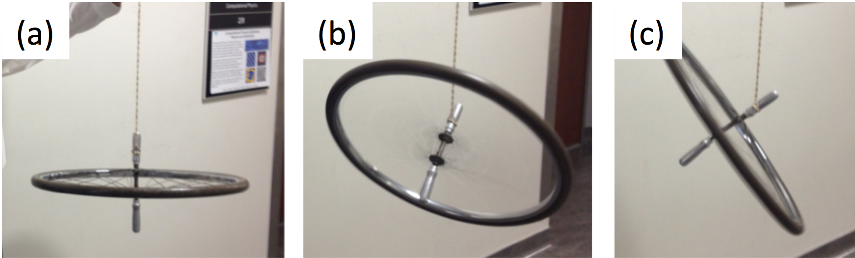
In the classical analog of precession, a spinning bicycle wheel experiences the force of the Earth’s gravitational field. (a) The precession cannot be measured when the spin axis is aligned with the Earth’s field. A torque is exerted onto the wheel, so that it precesses at an angle. At different moments in time, it will be in positions (b) and (c). The period to finish one rotation of precession is a characteristic time.
From a quantum mechanical approach, even a single proton is in a superposition state of spin-up and spin-down. The probability of finding the proton in the up or down state is given by the Boltzmann factor, see Eq.(6.5). In the mechanical analogue shown in Fig. 1.1, the equilibrium position corresponds to the first figure, when the Earth’s gravitational force is aligned with the angular momentum of the wheel - assume that the wheel is spinning. In order to visualize the precession, a mechanical kick is provided to tilt the wheel.
Similarly, it is necessary to torque the magnetic spin away from the main magnetic field \(\vec{B_0}\) direction. We will assume that this magnetic field points along the z-axis. Providing an electro-magnetic kick, the nuclear spin can precess and the time-changing moment induces a current through Faraday induction in a receiving coil that can be detected to deduce this precession.
How can the spin direction be changed? A secondary coil - aligned perpendicular to \(\vec{B_0}\) - may create a magnetic field \(\vec{B_1}\) to tip the spins over. Mathematically, a torque is created that is proportional \(\mu \times \vec{B_1}\). This pulse generates the non-equilibrium precession. The maximized pulse is called a \(\pi/2\) pulse corresponding to a pulse that lasts for one forth of a full rotation (\(2\pi\)). After a characteristic time, the spin falls back to its ground state, thereby changing the magnetic flux through a pick-up coil. The induced emf in the pick-up coil can be detected.
6.3 Larmor Precession
Most atomic nuclei have a magnetic moment \(\vec{\mu}\), a pseudovector. The magnetic moment can be split into two components, one part is given by the geometry and the second part can be controlled and is related to the spin. Combining Eqs.(6.1) and (6.2), the magnetic moment of a nucleus is the written as
\[\begin{equation} \vec{\mu} = \gamma \vec{I}, \tag{6.3} \end{equation}\]
where \(\gamma\) is the and the \(\vec{I}\) is the quantized angular momentum vector. Assuming that the angular momentum is along the z-axis, for example, we can write the quantization for the angular momentum as follows: \(I_z = m \hbar\), where \(m\) is a half-integer. For example, for \(I_z = \frac{1}{2} \hbar\), it follows that \(m\) can assume two values, namely \(\pm 1/2\).
As mentioned in Sec. ??, it would be difficult to control a single nucleus, therefore experiments are usually setup for a collection of spins called ensemble (typically \(> 10^{19}\)). A constant magnetic field \(\vec{B}_0\) is used to polarize the nuclei in a particular direction. On average, at finite temperature, not all spins will point into this direction, but a majority - determined classically by Boltzmann-Maxwell distribution - will orient themselves in that direction. Applying a secondary RF magnetic field perpendicular to the DC polarizing magnetic field would give the nuclei a "kick" to precess. This happens at a frequency referred to as the Larmor frequency.
Let us first realize that the magnetic moment of the nucleus \(\vec{\mu}\) experiences a force in the presence of a magnetic field \(\vec{B}\). Then, there will be a torque
\[ \tau = \mu B \sin \theta = \gamma I B \sin \theta \]
where \(\theta\) is the angle between the magnetic field and the direction of the spin. The precession means the protection of the angular momentum (\(I \sin \theta\)) is changing with time, namely that \(\Delta I = I \sin \theta \Delta \phi\), so that - using the conservation of angular momentum \(\vec{\tau} = d\vec{I}/dt\) - we can write
\[ \gamma I B \sin \theta = \frac{dI}{dt} = \frac{I \sin \theta \; d \phi}{dt} \]
so that we can determine the precession angular frequency \(\omega\), which is called the precessional or Larmor frequency
\[\begin{equation} \omega_{Larmor} = \frac{d \phi}{dt} = \gamma B \tag{6.4} \end{equation}\]
The gyromagnetic ratio of 1H is known to a very high precision, at least 10 digits, it is 42.57747852 MHz / T. Therefore, by measuring the resonance frequency, the magnetic field can be measured to extremely high precision. Experimentally, the frequency is best measured using a beat frequency method.
6.4 Acoustic Beat Frequency
The Larmor frequency is tuned using an acoustic phenomenon called beat frequency. In acoustics, two interfering frequencies create a beat, when the frequencies are close enough that they create amplitude variations (beating). Consider two signals with approximately the same amplitude and angular frequencies of \(\omega\) and \(\omega + \Delta \omega\), where \(\Delta \omega\) is small compared to \(\omega\). The sum of two frequencies can be written as
\[ \cos(\omega t) + \cos(\omega t + \Delta \omega t) = 2 \cos \left( \omega t + \frac{\Delta \omega t}{2} \right)\cos \left( \frac{\Delta \omega t}{2} \right) \]
Now, the beating becomes evident, as illustrated in Fig. 1.2.
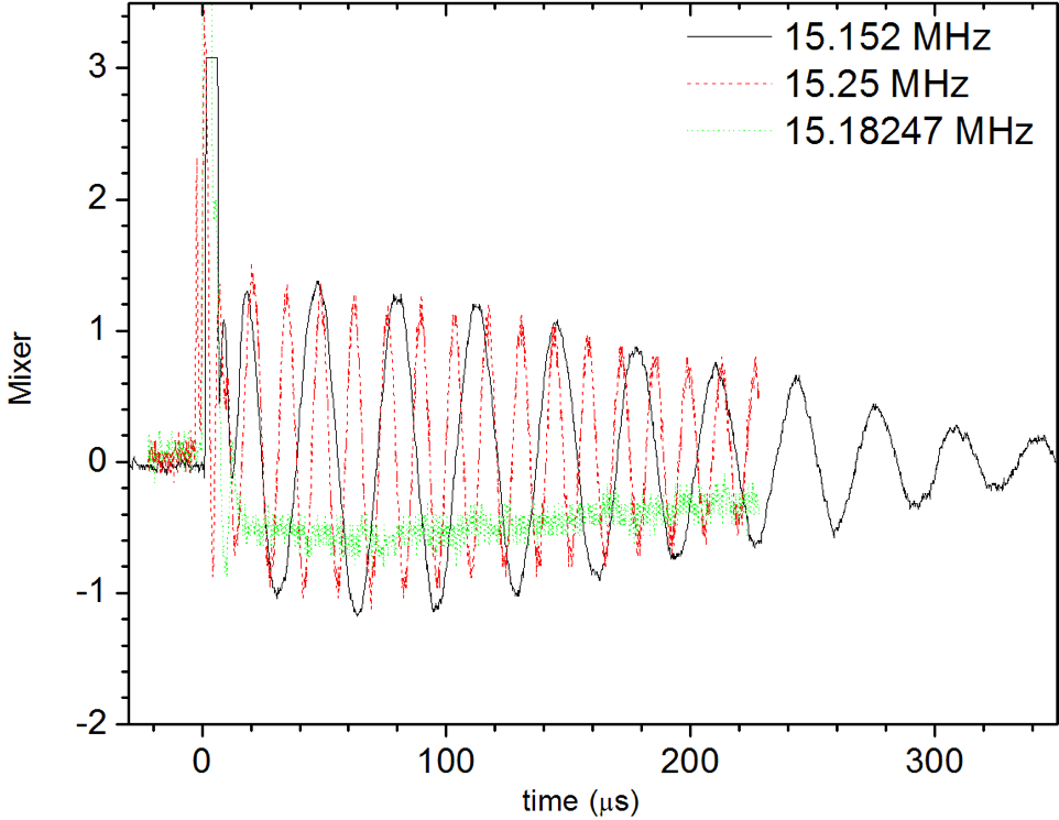
Experimental data for mixing a generated continuous wave rf signal with the detector signal of the free induction decay of glycerin.Two interfering frequencies are added with (a) 0.01% and (b) 0.2% frequency change. The total amplitude doubles as expected, however, there is a perceived variation in amplitude that corresponds to beats.
In pulsed nuclear magnetic resonance (PNMR), the interference pattern is created from two oscillating signals, the unknown experimental precession of hydrogen atoms and a known oscillator. An approximate value of the magnetic field can be used to compute the starting frequency for the oscillator, see Eq. (6.4). The signal from the oscillator is mixed with the electro-magnetic precession signal from the hydrogen atoms and viewed on an oscilloscope for example. In addition to the permanent magnetic field, a small transverse magnetic field \(\vec{B}_{ac}\) is used to start the precession of the hydrogen atoms, this short pulse needs to be repeated due to the decay of the precession.
6.5 Chemical Shift
For a macroscopic system that is in thermal equilibrium at temperature \(T\), the probability \(P_{E_i}\) of finding particles in a discrete energy state \(E_i\) is given by the , which is the exponent in the following equation.
\[\begin{equation} P_{E_i} = \frac{1}{Z} \exp \left( -\frac{E_i}{k_B T} \right) \tag{6.5} \end{equation}\]
Here \(1/Z\) is a normalization factor, where \(Z\) is commonly called the partition function (Zustandssumme). For a system with only two states \(P_{-}\) and \(P_{+}\), \(Z=\exp(-\frac{E_+}{kT})+\exp(-\frac{E_-}{kT})\). The condition to find the spin in anyone state is written as \(P(E_-)+P(E_+)=1\). Near room temperature, the spins of the hydrogen atoms in water, for instance, will randomly point up and down, with a tiny, tiny number of excess spins in one direction, when a magnetic field is applied. Only this spin difference \(\Delta N\) is relevant for the net polarization and it can be calculated as \(\Delta N = N_+ - N_-\), where \(N_+ = P_{+1/2} N\).
From one of the exercises using statistical physics, we find that the difference in number of nuclei with spin-up and spin-down is given by,
\[ \Delta N = N \frac{\Delta E}{2 k_B T}, \]
where \(N\) is the total number of atoms. The number of active nuclei, or signal strength, can be increased by going to lower temperature, by increasing the volume of material (\(N\)), or by increasing the energy gap (more magnetic field or higher gyromagnetic moment of the selected nucleus).
Using some typical numbers of \(B=1T\), and \(\gamma\) for \(^1\)H of 42.58 MHz/T, we have \(\Delta E \sim 0.2 \mu\)eV. Thus, we have for room temperature \(\Delta N / N \simeq7\cdot 10^{-6}\). Id est, for every million nuclei, there are 7 excess states in \(|+>\) compared to \(|->\).
Let \(P\) be the probability per unit time and per spin of a transition induced by a perturbation through a perpendicular magnetic field \(B_1\). Then, we can find the rate of transitions, which is \(R=P \Delta E \Delta N\). The detector coils actually measure the induced current from a magnetic flux change \(\Delta V = -d\Phi / dt\), and therefore the observed signal \(S\) can be written as,(Harris 1986)
\[ S \sim \frac{\gamma^4 B_0^2 N B_1 }{T} \]
We observe that there is a strong dependence on \(\gamma\), refer to Tab.1.2??. Also, high constant magnetic fields \(B_0\) are desirable to maximize the signal. The mangetic field should also be homogeneous across the sample. The signal strength is proportional to the sample size \(N\). The total signal can be increased further by lowering the temperature.
Importantly, the nucleus is somewhat shielded from the magnetic field \(B_0\) by the surrounding electrons, which create a magnetic field themselves. This shielding reduces the effective magnetic field at the nucleus’ location by a small fraction \(\sigma\), so that the detected effective magnetic field can be written as
\[ B_{\mathrm{eff}} = B_0 \left( 1-\sigma \right) \]
The Larmor frequency \(\omega = \gamma B\) may vary for the same nucleus in a given molecule depending on the bonds. Take the 1H spectrum of sec-butanol. Note that the magnetic fields of H-O and H-C bonds are different. Moreover, 5 different magnetic fields are distinguished, \(2\times\) CH3 (chirality), CH, OH, and CH2. When the magnetic field shift is translated to a measured frequency shift, it leads to what is known as a chemical shift. This chemical shift is generally measured with reference to a standard as it is much easier to measure a difference rather than an absolute value. One common standard is tetramethylsilane, Si(CH\(_3\))\(_4\), or TMS. The shift is then expressed in terms of \(\delta\), where \(\delta \equiv 10^6(\sigma_{\mathrm{TMS}}-\sigma_{\mathrm{sample}})\).
The shielding constant \(\sigma\) is the sum of three contributions. The first contribution \(\sigma_{loc}\) is due to the electrons on the atom that contains the nucleus; the second part \(\sigma_{mol}\) is the contribution from the other parts of the molecule that further shield the magnetic field. Additionally, the third part is shielding from the solvent, which may be used.
The local contribution is the sum of a diamagnetic and paramagnetic signal. The Lamb equation provides a way to compute the diamagnetic contribution
\[ \sigma_{loc,dia} = \frac{e^2 \mu}{3 m_e} \int _0^\infty \rho(r) r \; dr \]
In hydrogen, \(^1\)H, there is only 1 s-orbital, which implies that the diamagnetic contribution dominates and can be computed based on the electron density \(\rho(r)\). The computations quickly escalate and become complex. In practice, measured values of the shielding constant \(\sigma\) are often compared to known values using available tables and software.
6.6 Bloch Equations
For an ensemble or set of \(N\) nuclei, we define the polarization as \(\vec{M} = \sum \vec{\mu}_i\). In the presence of a magnetic field \(\vec{B}\), the nuclear spins can precess around this constant magnetic field. This can be mathematically realized by understanding the conservation of angular momentum, \(\tau = \frac{d \vec{I}}{dt}\) and using Eq.(6.3), we have
\[\begin{equation} \frac{d \vec{M}}{dt} = \gamma \left( \vec{M} \times \vec{B} \right) \tag{6.6} \end{equation}\]
Case 1: we solve this equation for \(\vec{M}(t)\) with the condition that the magnetic field is constant and aligned: \(\vec{B}_0 = <0,0,B_0>\). We find that the spin will precess forever:
\[ \frac{dM_x}{dt} = - \gamma M_y B_z = \omega_0 M_y \\ \frac{dM_y}{dt} = - \gamma M_x B_z = \omega_0 M_x \\ \frac{dM_z}{dt} = 0 \]
Therefore, the z-component of the magnetization is constant; i.e. \(M_z(t) = M_{0,z}\), given by the initial conditions. Multiplication of the second equation with the complex number i and adding them together with a substitution of \(Q \equiv M_x + i M_y\) and \(\omega_0=\gamma B_0\), we find that \(Q(t)\) is on a circular path with the Larmor frequency:
\[ \frac{d}{dt} Q = -i \omega_0 Q \]
with the solutions \(M_x(t) = M_{0,x} \cos(\omega_0 t)\) and \(M_y(t) = M_{0,y} \sin(\omega_0 t)\). Notably, the polarization along the x-axis will oscillate at the Larmor frequency and in 3D it will precess forever. In practice, this ideal situation is not observed due to interactions of the nuclear spins with the environment.
Swiss-born physicist Felix Bloch expressed this relaxation empirically by introduction of an additional term in the equations of motion, which can be expressed as a diagonal matrix \(\hat{R}\) with elements that have units of frequency (inverse time).(Bloch 1946) The diagonal elements can be interpreted as longitudinal and transverse characteristic frequencies:
\[ \hat{R} = \left( \begin{array}{ccc} \frac{1}{T_2} & 0 & 0 \\ 0 & \frac{1}{T_2} & 0 \\ 0 & 0 & \frac{1}{T_1} \end{array} \right) \]
He rewrote the Eq.(6.6) into a new equation, which is now known as the Bloch equation:
\[\begin{equation} \frac{d \vec{M}}{dt} = \gamma \left( \vec{M} \times \vec{B} \right) - \hat{R} \left(\vec{M} - \vec{M}_0 \right) \tag{6.7} \end{equation}\]
where \(\vec{M}_0\) is the equilibrium polarization. It means that the average spin vectors \(\vec{M}\) will eventually tend to go back to the ground state \(\vec{M}_0\). This ground state is aligned with the constant magnetic field \(\vec{B}_0\). It is given by the familiar Curie formula - assuming \(\mu B \ll k_B T\), always satisfied except for very low temperatures or extreme magnetic fields,
\[ \vec{M}_0 = N \frac{ \gamma^2 I (I+1)} {3 k_B T} \vec{B}_0 \]
Case 2: Similarly, Eq. (6.7) can be solved for the case of a constant and z-aligned magnetic field \(\vec{B}_0= <0,0,B_0>\). It follows that \(\vec{M}_0 = <0,0,M_0>\) has a z-component only, and simplifies to the following set of equations:
\[ \frac{dM_x}{dt} = \gamma M_y B_0 - \frac{M_x}{T_2} \\ \frac{dM_y}{dt} = -\gamma M_x B_0 - \frac{M_y}{T_2} \\ \frac{dM_z}{dt} = - \frac{M_z}{T_1} + \frac{M_0}{T_1} \]
The two relaxation times that were introduced can be understood as the spin-lattice relaxation \(T_1\) and the spin-spin relaxation \(T_2\). These interactions decay exponentially with the characteristic times \(T_1\) and \(T_2\). We solve Bloch’s equations in this case and find solutions with \(\omega_0 = \gamma B_0\)
\[\begin{equation} M_x(t) = e^{-t/T_2} \left( M_{0,x} \cos (\omega_0 t) + M_{0,y} \sin(\omega_0 t) \right) \\ M_z(t) = M_0 + (M_{0,z} - M_0)e^{-t/T_1} \tag{6.8} \end{equation}\]
From these equations, you can see that the z-component relaxes with the time constant \(T_1\), where as the x- and y- components are relaxing with a characteristic time of \(T_2\). Both equations are graphed in Fig. 1.3.
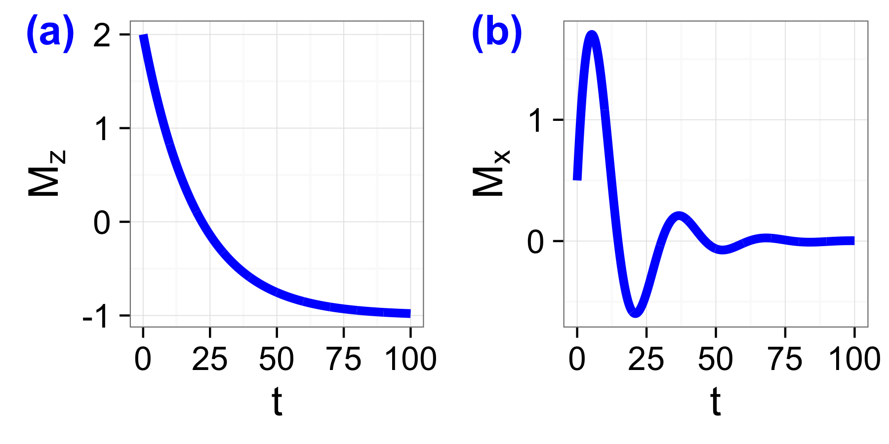
(a) Graph for \(M_z(t)\) for \(M_0 = -1\), \(M_{0,z}=2\), and \(T_1=20\) with no units according to Eq.(6.8), and (b) graph for \(M_x(t)\) using \(\omega=0.2\), and \(M_{0,x}=0.5\), \(M_{0,y}=2.5\).
Case 3: Most experimental setups, have a time-dependent field, where a secondary magnetic field is added to the polarizing main magnetic field \(\vec{B}_0\). Therefore, we should consider a time-dependent magnetic field \(\vec{B} = < B_1 \cos(\omega t) , B_1 \sin(\omega t), B_0>\). This would be the point-of-view of the laboratory or rest frame. In the reference frame of the rotating \(\vec{B_1}\) field, we can eliminate the time-dependence, but now the effective field in z-direction would be reduced. Since, we are spinning in the x-y plane of this reference frame, the magnetization \(\vec{M}\) appears static.
Thus, in the rotating frame, the magnetization \(\vec{M'}\) is given by the magnetization \(\vec{M}\) as follows:
\[ \frac{d \vec{M'}}{dt} = \left( \gamma \vec{B} - \vec{\omega} \right) \times \vec{M} \]
Therefore, the torque must vanish, since there is no change of the magnetization: \(\tau = \frac{1}{\gamma} \frac{d\vec{M'}}{dt} = \vec{M} \times \vec{B'} = 0\). The effective magnetic field \(\vec{B'} = \vec{B_0} - \vec{\omega}/\gamma\) will guide the precession. Imagine, that this effective field in the z-direction becomes zero, so we have the condition that \(\omega/\gamma = B_0\). Now, we provide just the right frequency \(\omega = \gamma B_0\) for the z-component to vanish, then we have only the \(B_1\) field in the rotating frame; for our purposes, we fix the direction along the x-axis, such that the magnetic field is \(\vec{B}_{eff} = B_1 \hat{x}\) As soon as the \(B_1\) field is turned on, or the pulse is generated, a precession of the magnetization \(\vec{M}\) in the y-z plane commences. The frequency of this precession is \(\Omega = \gamma B_1\). Note: \(B_1 \ll B_0\), since \(B_1\) should not polarize the sample; therefore, \(\Omega \ll \omega_0\) If the pulse is finite in time, the direction of the magnetization can be “stopped” in the rotating frame, for example with a \(90^o (\pi/2)\) pulse, the magnetization will be directed along the y-axis. Similarly, a \(180^o (\pi)\) pulse would direct the magnetization in the -z direction. The magnetization would return back to the +z direction with a \(360^o (2\pi)\) pulse.
For any angle other than \(n\pi\), where \(n\) is an integer, the non-equilibrium magnetization will relax back to the thermal equilibrium. This change in magnetization induces a voltage that can be picked up. It is called the free induction decay (FID) signal.
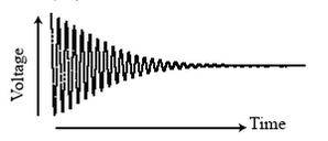
Free induction decay voltage picked up by the detector coil after a pulse set the nucleus spins out of equilibrium.
6.7 Pulse Sequence
The principle of nuclear magnetic resonance is the ability to excite nuclear spins with radio frequency pulses. When the nuclei revert back to equilibrium, they emit RF radiation that is detected. The signal contains the unique signature of the nuclear spin energy gap.
Given the frequency of a proton in the presence of a strong magnetic field, precession can occur if a pulse of accurate length is applied at the proper frequency to the sample. The resonance frequency is tuned by mixing the RF sample signal with a continuous wave (CW) RF signal. If the frequency from the sample is out of tune, a beating pattern will be observed. Changing the frequency allows the complete elimination of the beating and ensures that you are at resonance frequency. That frequency changes due to the change in temperature in the room, which affects the magnetization of the permanent magnet that polarizes the sample.
At resonance frequency, pulse sequences are used to probe the sample. The simplest pulse is a 90° pulse. Here, the angle corresponds to a particular time, which is related to the resonance frequency. Therefore, the 180° pulse is twice as long. In the mechanical analogue, consider a swing: the resonance frequency of the swing is given by the length of the swing rope and the mass of the Earth. Your friend asks you to swing them higher, so increase the amplitude. First of all, your push needs to have the same frequency as the resonance frequency of the swing; it also needs to be in phase. Lastly, you can push for different amount of lengths. If you swing from the highest point, to the lowest point, it would correspond to a 90° pulse.
Using the pulse generator, the pulse is programmed and submitted as an RF pulse to the sample. The oscilloscope is triggered at the beginning of the pulse and subsequent pulses are spaced by the repetition time, which must be large enough to avoid overlap - take a moment to understand that. The precession is maximal at 90°, therefore the signal that is picked up, also called the free induction decay, will have a maximum at 90°. For a rotation of 180° there is no precession, the nuclear spin was simply reversed from the direction of the strong magnetic field and will decay back in sufficient time. However, 270° will again produce a maximum signal. Technically, there is a phase difference, however in the experimental setup, generally only the amplitude is detected, therefore a 90° and 270° pulse will look alike. Still, you can distinguish the two pulses by continuously increasing the time and noting the number of the peak. The first maximum corresponds to a 90° peak, while the first minimum is a 180° degree pulse. This can be confirmed using the oscilloscope and explicit measurement of the time of each pulse.
The spin-lattice relaxation time \(T_1\) is measured using a 180° - \(\tau\) - 90° sequence, where the delay time \(\tau\) is varied. For very small delay times (\(\tau \ll T_1\)), the free induction decay maximum voltage measured after the second pulse (90°) will have a value similar to measurements when the delay time is very long (\(\tau \gg T_1\)). At intermediate delay times the free induction decay signal vanishes. This happens essentially in the situation when you reverse the polarization of the nuclear spin with the 180° and wait long enough for the majority to relax half-way back to the equilibrium position to apply a 90° peak, the spins will not precess.
For the spin-spin relaxation time \(T_2\), the measurement is opposite. Here the 90° - \(\tau\) - 180° sequence is applied. In the so-called Carr and Purcell pulse sequence (Carr and Purcell 1954), several consecutive 180° pulses are applied with the timing, such that the temporal space between 180° pulses is exactly twice the time \(\tau\) from the 90° pulse to the first 180° pulse. Some time after the second pulse, namely \(\tau\), there is an echo, known as first detailed by . The voltage amplitude of that echo relative to the original peak gives an estimate of how many spins have not yet lost phase. The amplitude of the spin echoes decreases exponentially with the time constant of \(T_2\). The spin-spin relaxation time \(T_2\) has to be smaller than the \(T_1\) .
Experimentally, the spin-spin relaxation measurements uses a long sequence of 180° pulses. If the pulse is not precisely 180°, then the error is propagated and after 10 – 30 pulses leads to significant errors. A solution to this problem was given by Meiboom and Gill.(Meiboom and Gill 1958) They use the Carr and Purcell pulse sequence, but after the first pulse, a phase shift of 90° is introduced. This shift is relative to the original 90° pulse and with respect to the following 180° pulses. Secondly, successive pulses are coherent, which means that the direction of the RF pulses creating the small magnetic field is the same for all pulses.
6.8 Magnetic Resonance Imaging
The scanner allows a 3D view of the internal structure of the human body. It is based on nuclear magnetic resonance and adds spatial resolution to it. The spatial resolution is obtained through that fact that the resonance frequency changes with the magnitude of the applied magnetic field (refer to Eq.??). If a magnetic field gradient is produced, the spatially varying magnetic field will produce a spectrum of frequencies. The intensities would vary depending on the number of spins with that particular resonance frequency. Using a Fourier analysis, it is possible to deconvolve this signal and produce a 2D spatial image, which if repeated can produce a 3D view of the sample or human body.
The time-varying magnetic fields, or microwaves, can heat the body just like a microwave. A precise calculation is on order, but a general rule of thumb is that a specific absorption rate (SAR) of 4 W/kg causes the core temperature to rise by 1°C(Freeman 2003).
In the early 1970s, it became clear that NMR can be used to detect malignant tissue.(Damadian 1971) In x-ray diffraction, the contrast scales with the square of the atomic number (\(\sim Z^2\)), so that high-density material (calcium in bones) can be easily analyzed. On the other hand, NMR can be tuned to the frequency of hydrogen and probe soft tissues, such as gray and white matter, muscles, fluids, and fat. The majority of the human body is composed of water and fat and other hydrogen containing molecules. The hydrogen nucleus has a very high gyromagnetic ratio, so that high sensitivity can be obtained. In addition to the general setup for NMR, magnetic resonance imaging (MRI) uses an additional gradient magnetic field.
The strong constant magnetic field polarizes the nuclei. At room temperature, far from all spins are aligned with the magnetic field. Typically, about half the spins are aligned, and the other half are anti-aligned, and it is only the small excess of nuclei (about one in a million), which point in the direction of the magnetic field that contribute to the MRI signal. On top of this strong constant field, a magnetic field gradient is applied, so that the magnetic field at the top is slight different as opposed to at the bottom. A secondary magnetic field perpendicular to the first magnetic field, provides the 90° pulse for the nuclear spins to start precession. The spin-lattice relaxation ensures that the precession will vanish after the characteristic time \(T_1\), which is 500 ms–900 ms for brain matter. During this relaxation time, RF radiation corresponding to the Larmor frequency is emitted and detected via an RF coil.
The detected RF signal would be composed of a single frequency, if the frequency were the same for all nuclei. However, the gradient magnetic field created different Larmor frequencies in space, according to \(\omega_0 = \gamma B\). A Fourier transform of the signal will reveal all the frequencies in the signal. Those frequencies can be mapped to known locations, revealing a density map. For example, white matter has a lower \(T_1\) than black matter in the brain. Since the white matter is located at a different position, the signal is encoded in the frequency. A computer can then generate the two-dimensional image, and even create a three-dimensional image after successive repetitions in different slices of the body.
For MRI, typical magnetic fields of 1.5 T are achieved in a space that the human body can fill. Therefore, large currents are needed to produce the magnetic field. The dissipation in regular wires would produce too much heat. So, only superconducting magnets can be used. They require constant cooling by emersion in liquid helium. The discovery of high-temperature superconductors by German J. Georg Bednorz and Swiss K. Alex Müller allowed for much more economical ways of running super currents used in MRI, since cooling by liquid nitrogen is sufficient. Once the current is established, it will run without dissipating any heat; the power in an MRI machine is simply used to keep the nitrogen or helium cool.
The gradient magnetic field is applied in two directions. For the following example, we will examine only one gradient magnetic field, so that the magnetic field has the following form:
\[ B(z) = B_0 + G_z z \]
it follows that the frequencies are given by \(\omega(z) = \omega_0 + \gamma G_z z\). The signal will have the following form: \[ s(t) = \int_{-\infty}^{\infty} m(z) e^{-2\pi i \left( \frac{ \omega_0 + \gamma G_z z}{2 \pi} \right) t } \; dz \] it can then be rewritten in the form that the carrier frequency \(\omega_0\) becomes clear.
\[\begin{equation} s(t) = e^{-i \omega_0 t} \int_{-\infty}^{\infty} m(z) e^{-2\pi i \left( \frac{ \gamma G_z z}{2 \pi} \right) t } \; dz \tag{6.9} \end{equation}\]
The function \(m(z)\) can be obtained by applying the inverse Fourier transform. In reality, this is performed with the fast (FFT) algorithm. An image is then generated. Eq.(6.9) shows how the time domain is converted to space domain. A signal with more time, therefore will give more spatial resolution. For organs that move, such as the heart or lungs, complicated trigger schemes must be invented, in order to produce a long time signal for sufficient spatial resolution.
6.9 Quantum Computing
Quantum computing allows for very fast execution of parallelized code, such as prime factoring or sorting algorithms (Shor 1997). For quantum computing, a qubit is the lowest unit and can be implemented in several systems, such as with quantum dots, ion traps, and NMR. The advantage of NMR is the long coherence time measured as T\(_1\) (logitudinal) and T\(_2\) (transverse) time constants. T\(_1\) is also called spin-lattice time, or amplitude damping, and T\(_2\) is called spin-spin relaxation time, or phase damping. In general, T\(_1 >\) T\(_2\). A quantum computation should be finished before a state has become decoherent.1 The implementation of quantum computing with NMR involves single-spin rotations (Vandersypen and Chuang 2005).
6.10 Books
Many books have been written about nuclear magnetic resonance. There are also online open-texts, such as Joseph N. Hornak, "The Basics of NMR", http://www.cis.rit.edu/htbooks/nmr/.
6.11 Problems
What is the nuclear spin \(I\) of the hydrogen atom, \(^7\)Li, \(^{13}\)C, \(^{15}\)N, \(^{19}\)F, and deuterium?
How many possible energy states does \(^{27}\)Al with \(I\)=5/2 have? What about \(^{59}\)Co with \(I\)=7/2?
Name three nuclei with zero nuclear spin; i.e. \(I=0\).
What is the direction of the magnetic moment to have the lowest energy, which configuration has the highest energy?
The Earth’s magnetic field is relatively homogeneous over large areas. Calculate the resonance frequency of a proton.
Calculate \(\Delta E\) for a proton immersed in a typical B-field of 2.35 T. Then, determine the ratio of \(\Delta E\) with \(k_B T\) at room temperature.
Calculate a typical value of \(\Delta N\) for a system of protons at room temperature with N=10\(^6\).
Calculate the susceptibility \(\chi\). Note that the Curie equation is \(M=\chi/T\), where \(M\) is the total magnetization. Express your answer in terms of \(\gamma\) and the constant magnetic field \(B_0\).
Explain why water can be treated as protons only in the case of NMR. And what about mineral oil?
What is the resonance frequency of sodium in a magnetic field of 1.6 T?
References
A TNC (threaded Neill-Concelman) connector is similar to a BNC (Bayonet Neill-Concelman) connector, but instead of a twist it has a thread that is screwed in. The TNC is superior in performance at microwave frequencies.\[TNC\]↩︎