Chapter 7 AFM
7.1 Introduction
Quantum tunneling had been known as a phenomenon in radioactivity since the late 19th century. In the late 70s, Gerd Binnig with Heinrich Rohrer at IBM Rüschlikon, Switzerland, and later along with technician Christian Gerber and then Edi Weibel started building what would become the first scanning tunneling microscope (STM) (Gerd Binnig and Rohrer 1987).
In March 1981, tunneling through a vacuum barrier was controllably shown to have the characteristic form of the logarithmic current with distance and importantly their slope being equal to the tunnel barrier height (G. Binnig et al. 1982).
A similar concept of the tip-sample probe was also built by Russel Young from NIST, USA, and he realized that with tunneling currents small features could be measured, however, edificial vibrations were an issue in constructing the setup. To overcome the vibration issue, the Swiss research team built their station on top of a magnet which was elevated via a superconductor, thus avoiding vibrations. Using piezoelectric materials, the lateral position can now be be adjusted to 200pm and the vertical position to 10pm.
Only 1 year later, Tersoff and Hamann from Bell Laboratories in New Jersey developed the theoretical background to model the experimental data that allowed for the first time to probe non-periodic atomic structures.(Tersoff and Hamann 1983)
Initially, the making of a sharp tip represented some challenges. One method is to attach strings with weights on each end of the tungsten filament. An infrared laser is used to melt the tungsten in a point as the weights pull the filament slowly apart. A sharp tip emerges.
This scanning tunneling microscope (STM) had limitations as it was based on an electrical tunneling current. It required good vacuum, low temperatures, and most of all conducting samples.
A few years later, Binnig and Gerber started a collaboration with Quate at Stanford in California to build a more general machine, the atomic force microscope (AFM) was devised.(G. Binnig, Quate, and Gerber 1986) This development was driven by the high precision of moving the tip. Rohrer mentioned it could be positioned with a range of 10pm, now keep in mind that the orbital size difference between an isolated hydrogen atom (n=1) and its excited state (n=2) is about 160pm. This extraordinary spatial precision is based on the piezoelectric effect.
Operating the AFM at room temperature, one can measure forces as small as 1 fN, at sub-Kelvin temperatures forces as small as 1 aN can be detected.
The first AFM had a Q factor of only about 100, and used a cantilever with a relatively low resonance frequency of 5.8kHz. One issue - immediately recognized - was thermal drift issues and other effects that reduce the repeatability and reproduction of a particular sample. In their first AFM experiment, they used a 25 μm thick and 800 μm long gold foil cantilever with a diamond tip.
In 1986, Gerd Binnig and Heinrich Rohrer received the Nobel prize for their design of the scanning tunneling microscope. The prize was shared with Ernst Ruska who built much earlier in 1933 the first electron microscope.
The AFM image is artificially colored, but it also represents a convolution of the tip’s image and the surface morphology. Therefore, the tip can affect the shape and image.(Abraham, Batra, and Ciraci 1988) Moreover, the tip can also interact with the sample, such that the surface is disturbed or modified. This can also happen to the tip itself. For example, for silicon, a force of less than 1 nN should be applied to avoid disturbing the sample surface.
The AFM can be operated in air, vacuum, or liquids. The latter allows imaging of DNA and proteins absorbed on a surface. Pure water should be avoided as the behavior gets complex; rather ethanol should be used.(Weisenhorn et al. 1992)
Naturally, AFM can be used to intentionally modify the surface. Techniques have been developed specifically for nanolithography and nanoindentation. Individual atoms can be lifted off by applying a force; this is a purely mechanical response (Oyabu et al. 2003).
7.2 Objective
Atomic force microscope (AFM) is an extremely versatile tool for characterization of nanotechnology, see the review by Giessibl (Giessibl 2003). The AFM is a special type of Scanning Probe Microscope (SPM). In 1981 Gerd Binnig and Heinrich Rohrer realized the first scanning tunneling microscope (STM) at IBM Rüschlikon in Switzerland, which works on conducting samples by scanning a smooth surface at low temperatures with a Pt:Ir probe that is atomically sharp (G. Binnig et al. 1982). The probe is approached such that tunneling currents between the sample surface and the probe can be measured. Quantum mechanics make the tunneling current extremely distance dependent. Thereby scanning the surface at constant current a precise topography image is obtained. A few years later, the AFM was developed to probe non-metallic surfaces as well. At the time, (G. Binnig, Quate, and Gerber 1986) demonstrated 3 nm lateral resolution and less than 1 Å vertical resolution; i.e. individual atoms are resolved. Nowadays, the AFM is used by scientists, researchers, and engineers for quality control and fundamental research alike.
At the end of this experiment, you will be able to setup a commercial AFM, take basic topographical images, and analyze AFM images. The goal shall include a basic understanding of the concepts for atomic force microscopy and provide a beginner’s tutorial for using the equipment. Understanding the precise operation of the different AFM models is important in order to take high-quality images and to properly analyze the images.
This section will introduce you to some of the capabilities of atomic force microscopy, its applications in science, research, and industry, and detail the procedure to scan surfaces at sub-visible resolution. Visible light is an electromagnetic wave with wavelength \(\lambda= 390 - 770\) nm. Therefore, features that are smaller than the diffraction limit cannot be easily resolved with optical light.
Nanotechnology has broad inter-disciplinary applications that include computing, data storage, health, energy storage, new displays, and bio-, gas sensor applications based on Gold nanoparticles, carbon tubes, self-assembly, and nanotubes. In order to understand and explore these devices, it is important to probe at length scales much below one micrometer. Atomic force microscopy is one of many probing techniques suitable for probing nanotechnology.
It is important to note that an AFM image does not represent the sample topography, but rather it is a convolution of the scanning tip and the sample topography. Each tip is nanoscopically different and therefore interacts uniquely with the sample. The interaction between the tip and sample creates the image. The image may also contain artifacts of the scan head (contortions), vibrations, interference of the laser, and the image processing .
7.3 Attractive Forces
Surface morphology, electrostatic, and magnetic information at the nanoscale are explored using an AFM. The probing mechanism is similar to an old phonograph. In AFM, a very sharp (ideally atomically sharp) tip is dragged across the surface to measure a force of interaction between the surface and the tip. In vacuum, there are short-range chemical forces (fractions of nm) and van der Waals , electrostatic, and magnetic forces with a long range (up to 100 nm). In ambient conditions, meniscus forces formed by adhesion layers on tip and sample (water or hydrocarbons) can also be present. The van der Waals interaction is caused by fluctuations in the electric dipole moment of atoms and their mutual polarization. When a neutral object is polarized by the electric field of a charge, the resulting force is \(F \sim \frac{1}{r^2}\frac{1}{r^3}\), creating a potential that falls off with distance to the sixth power. A neutral object is always attracted. The van der Waals potential energy can be modeled as an attractive interaction with \(V_{vdW} = - A / r^6\), where \(r\) is the distance between the two objects. Only at very close distances, the repulsive forces of the atoms play a dominant role; these forces can be modeled loosely as \(V_{rep} = B/r^{12}\). The sum of these contributions is described by the Lennard-Jones potential
\[ V_{LJ} = - \frac{A}{r^6} + \frac{B}{r^{12}} \]
proposed in 1925. The function is graphed in Fig. ??. The reader may be reminded of the contributions from van der Waals for the non-ideal gas: the excluded volume constant provides a short-range repulsive force that is balanced by long-range attractive force introduced in the pressure modification. Here, the van der Waals force is a short-range force. The origin is found in fluctuations of the electron cloud surrounding the nucleus of electrically neutral atoms. For argon gas, the constants are best determined to be \(A= 1.02^{-77} Jm^6\) and \(B=1.58^{-134}Jm^{12}\).
In the case of AFM, this force is quantified with the Hamaker constant \(H\), given the tip radius \(R\) and the distance \(r\) of the sphere from the surface, then:
\[\begin{equation} V_{H} \sim - \frac{H R}{12 r} \end{equation}\]
with typical values of \(H\) in the range of \(10^{-19} - 10^{-20}\) J.

Lennard Jones potential for \(A\)=1 and variable \(B\) values and unit-less distance \(r\). The potential well models the sample-tip interactions. At large distances, the force is attractive (electrostatic), whereas at short distances, the force is repulsive (positive values). In non-contact mode, the AFM tip is operated at large slopes of the attractive regime. In contact mode, the tip is approached to the repulsive area.
The force is the slope of the potential. A negative slope at high \(r\) values corresponds to an attractive force, whereas a positive slope at low \(r\) values is a repulsive force.
In ambient air, surfaces are covered with a film of water. Therefore, as the tip approaches the sample surface, it will interact with water. The humidity of the room plays a role in the thickness (Butt, Cappella, and Kappl 2005). Sharp tips experience less influence from the water. A typical tip radius is about 8 nm, but varies with type and manufacturer.
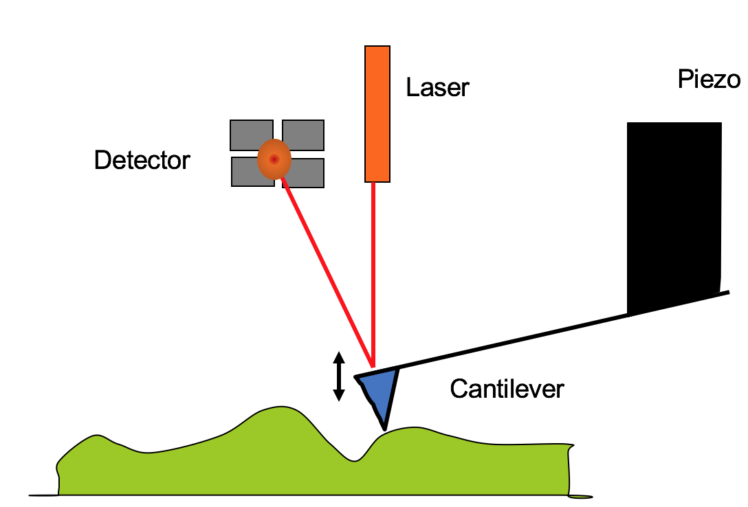
Schematic diagram of simple atomic force microscope.
There are different modes of AFM operation (static and dynamic are of main interest) with the basic idea of a feed-back loop that records the height, see Fig. ??. In static mode, the cantilever makes contact with the surface. In dynamic mode, on the other hand, the cantilever is positioned a few nanometers above the sample surface and oscillates at its resonance frequency. If the resonance frequency changes, the height is adjusted to keep the amplitude or force constant. The cantilever is attached to the AFM tip and the height is controlled with piezoelectric tubes. There are three tubes that are arranged to give full three-dimensional control, although only the z-control is shown in the simplified diagram. The interaction between the surface and the tip is measured via a reflected laser beam off the back of the cantilever. The detector generally has photodiodes that measure the light intensity via four separate detectors. By comparison of the top-down and left-right ratios, the offset from the central position indicates the strength of the force. The piezo will then adjust the height so that the laser beam is reflected back to the center. The motion of the piezo is referred to as the height.
By rastering the image left-right quickly and top-down slowly, a topographical image is created. The image has a typical resolution of 256 by 256 points or more. It may take several minutes to record an image depending on sample roughness and image size. The scan rate is reduced for larger areas in order to preserve the tip. The maximum scanning area depends on the scan head and should be noted carefully, as exceeding the range could damage the piezo-electric element. For the NanoSurf EasyScan the maximum size is 50\(\mu\)m, and for the NanoScope III, the tall scan head’s maximum range is 10\(\mu\)m. Before use of a new scan head, the piezo materials need to be calibrated.
The AFM tip, see Fig.~??, is at the end of a flexible cantilever. The cantilever is usually an “I” or “V” beam depending on the required resonance frequency. The cantilever is attached to a larger chip (standard is 1.6mm \(\times\) 3.4mm) in size. The cantilever is defined by a wet anisotropic etch and usually on the order of 40\(\mu\)m wide, 4– 8\(\mu\)m thick, and has a spring constant \(k\) of 0.1-10 N/m. The resonance frequencies can vary from 10 – 300 kHz. For quantitative measurements it may be necessary to know the spring constant of the cantilever. There are several ways to measure the spring constant \(k\) (Proksch et al. 1996), (Gredig 1998). The spring constant is related to both the geometry and the material (Young’s modulus). Two possible approaches include:
- Using the Euler-Bernoulli beam theory, an approximation for a rectangular cantilever of width \(w\) is made when knowing its thickness \(t\), the Young’s modulus \(Y\) and the length of the cantilever \(l\). In this case,
\[\begin{equation} k = \frac{Y w t^3}{4l^3} \end{equation}\]
- The image of the free vibration in air from a cantilever are due to thermal vibrations. If no other forces act on the cantilever, then the mean square of the amplitude \(<x^2>\) can be measured and using the equipartition theorem, the spring constant \(k\) is,
\[\begin{equation} k = \frac{<x^2>}{k_B T} \end{equation}\]
Such measurements are suitable for low spring constants and can be made with an uncertainty of about 10%. It is evident that the resonance frequency of the cantilever is a function of temperature.
Two similar tips will have slightly different resonance frequencies due to microscopic variations of the cantilevers’ shapes. The back surface of the cantilever should be reflective, so that a laser beam can be bounced off easily. Manufacturers often coat the back-side with Aluminum or Gold to improve the signal. The absolute value of the signal depends on the device itself, but typical values for the Park XE7 are 3V and for the Cypher AFM 8V, if the tip is reflective. The total signal, also called the sum signal should be maximized before tuning the cantilever.
The AFM image is always a convolution of the tip and the sample. Therefore, using different tips (even if the same type from the same manufacturer) will result in differences in the image. Some tips may lead to strong artifacts in the images. So-called “double tips”, for example, result in images that have periodic duplicates of structures or preferential directions in isotropic samples, such tips may be formed after collision with the sample. If it is suspected that the tip has a double tip, then it should be replaced, or the sample’s angle needs to be changed. This can be done by rotating the sample, going to a different position, or changing the scan angle.
In the static mode, the cantilever deflection is measured as the cantilever makes contact with the sample. The detector’s voltage signal is proportional to the tip sample force F = -∂V/∂z, where \(V\) is the potential energy. In the dynamic mode the cantilever is operated at its resonance frequency (usually 150-350 kHz). It is usually operated in constant amplitude mode; i.e. adjustments to the z-position are made in order to keep the resonance amplitude constant at all times. This system can be modeled with a driven damped harmonic oscillator, where the amplitude is modified by an interactive force between the tip and the sample.
7.4 Driven Damped Harmonic Oscillator
The AFM tip in contact with the sample surface can be modeled and understood as a forced damped harmonic oscillator. First, the cantilever, as discussed earlier, has a natural resonance frequency owning to its geometry. Using the momentum principle (Newton’s second law), we can write the differential equation for a harmonic oscillator,
\[\begin{equation} m\frac{d^2 x}{dt^2} + kx = 0. \end{equation}\]
The Ansatz for this differential equation is \(x(t) = e^{\lambda t}\), which leads to the solution that \(\omega_0^2 = k / m\). Therefore, the natural frequency of a cantilever of mass \(m\) and spring constant \(k\) is
\[\begin{equation} \omega_0 = \sqrt { \frac{k}{m} }. \end{equation}\]
The temporal solution would be \(x(t) = A e^{i\omega_0 t} + B e^{i\omega_0 t}\), where the amplitudes \(A\) and \(B\) are determined from boundary or initial conditions. The damped harmonic oscillator has a restoring force that is proportional to the velocity, i.e. we can write it as \(F_{r} = - \alpha v(t)\). The one-dimensional damped harmonic oscillator differential equation is written
\[\begin{equation} m\frac{d^2 x}{dt^2} + \alpha \frac{dx}{dt} + kx = 0. \tag{7.1} \end{equation}\]
This equation can again be solved with the same Ansatz, namely \(x(t) = e^{\lambda t}\), which leads to the following equation
\[\begin{equation} \left[ m \lambda^2 + \alpha \lambda + k \right] e^{\lambda t} = 0. \end{equation}\]
We will set the first term to 0 in order to solve the equation. The quadratic equation has two solutions,
\[\begin{equation} \lambda_{\pm} = \frac{-\alpha \pm \sqrt{\alpha^2 - 4 m k} }{2 m} \end{equation}\]
If we define, \(\beta \equiv \alpha / (2 m \omega_0)\), then we have \[\begin{equation} \lambda_{\pm} = -\beta \omega_0 \pm \omega_0 \sqrt{\beta^2 - 1} \end{equation}\]
The solution can be written as follows and the amplitudes \(A\) and \(B\) are determined from boundary conditions,
\[\begin{equation} x(t) = A e^{\lambda_+ t} + B e^{\lambda_- t} \tag{7.2} \end{equation}\]
We distinguish three different regimes, namely
- \(\beta > 1\): overdamped
- \(\beta = 1\): critically damped
- \(\beta < 1\) and \(\beta > 0\): underdamped
Note that for \(\beta=0\), we get an undamped harmonic oscillator with \(\lambda_{\pm} = \pm i \omega_0\). In the following discussion, the underdamped harmonic oscillator will be important. In this case, \(\beta\) is a small positive value. Commonly in AFM, the quality of the cantilever is measured using the Q factor, which is related as \(\beta = 1/(2 Q)\). Therefore, in the underdamped case, \(Q > 1/2\). The solution for the one-dimensional damped harmonic oscillator is
\[\begin{equation} x(t) = e^{-\beta \omega_0 t} \left [ A_0 \cos (\omega_{\gamma} t + \phi) \right] \tag{7.3} \end{equation}\]
The newly introduced frequency \(\omega_{\gamma}\) is called the ringing frequency, or damped frequency. It is a constant. Typical curves for this equation are shown in Fig.@(fig:DampedOscillatorPosition). The maximum oscillation amplitude decays over time as
\[\begin{equation} A(t) = A_0 e^{-\beta \omega_0 t}. \end{equation}\]
Using the solution Eq.(7.3) and inserting it back into Eq.(7.1), one quickly finds
\[\begin{equation} \left[1 - 2 \beta^2 + \left( \beta^2 - \frac{\omega_{\gamma}^2}{\omega_0^2} \right) \right] A_0 \omega_0^2 e^{-\beta \omega_0 t} \cos (\omega_{\gamma} t + \phi) = 0 %+ \\ % \left[ 2 \beta \omega_0 \omega_\gamma - 2\beta \omega_0 \right] A_0 e^{-\beta \omega_0 t} \sin (\omega_{\gamma} t + \phi) = 0 \end{equation}\]
The first term will vanish, when the ringing frequency \(\omega_\gamma\) assumes the following relation
\[\begin{equation} \omega_\gamma = \omega_0 \sqrt{1 - \beta^2} \end{equation}\]
For high quality factors \(Q\), the ringing frequency is close to the resonance frequency.
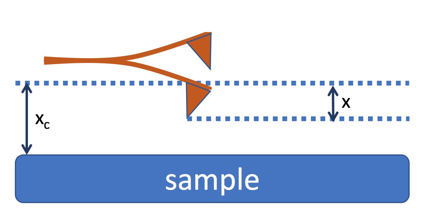
In dynamic mode, the cantilever is offset a distance \(x_c\) from the sample surface. The cantilever oscillates about that center position.
The AFM continuously delivers energy to the cantilever, so that we have a forced damped harmonic oscillator, which follows this differential equation
\[\begin{equation} m\frac{d^2 x}{dt^2} + Q\frac{m}{\omega_0} \frac{dx}{dt} + kx = k A_{exc} \cos \left( \omega_{exc} t \right) \\ \frac{d^2 x}{dt^2} + \frac{\omega_0}{Q} \frac{dx}{dt} + \omega_0^2 x = \omega_0^2 A_{exc} \cos \left( \omega_{exc} t \right), \end{equation}\]
where \(A_{exc}\) is the driving amplitude. Notice that the electronic analogue is a LRC circuit. The battery is the driving force.
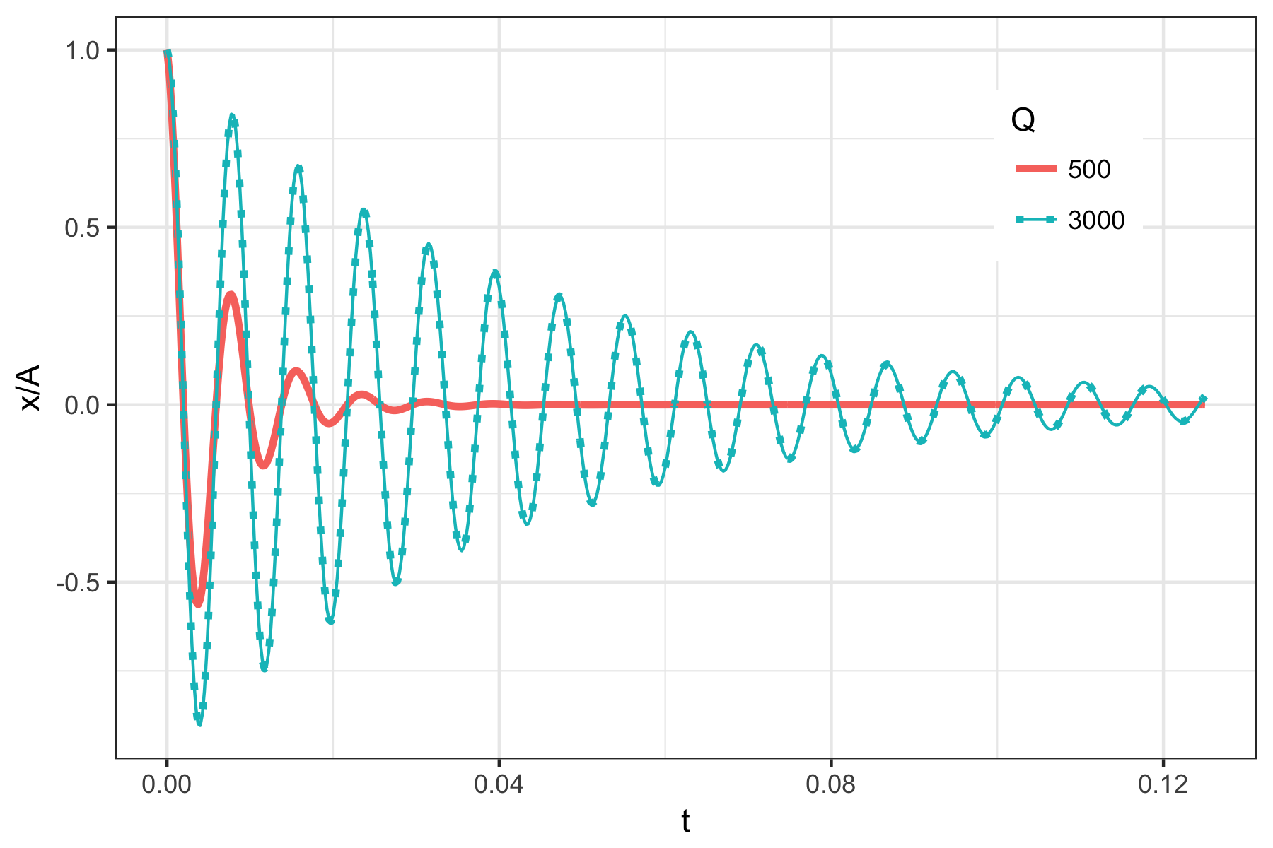
Damped harmonic oscillator’s position as a function of time with \(\omega_0\) = 150 kHz and \(Q\) = 500 or 3000. The lower quality factor means that the oscillations are damped more quickly.
As the cantilever gets close to the sample surface, there is an additional force presence, and we can write the differential equation of a dynamic cantilever tip as follows
\[\begin{equation} \frac{d^2 x}{dt^2} + \frac{\omega_0}{Q} \frac{dx}{dt} + \omega_0^2 x - \left[ \omega_0^2\frac{F_{ts}(t)}{k} \right] = \omega_0^2 A_{exc} \cos \left( \omega_{exc} t \right), \tag{7.4} \end{equation}\]
where \(F_{ts}\) is the tip-surface interaction and it is a function of the distance from the sample surface, so \(F_{ts}(x_c+x)\). In order to remove the time-dependence from \(F_{ts}\), we assume for small amplitudes the sample-tip force can be Taylor expanded. In this case, \(F(x_c + x) \approx F(x_c) + \frac{\partial F}{\partial x} |_{x=x_c} x + \ldots\) and we can define a new spring constant \(k^{'}\)
\[ k^{'} = \frac{\partial F}{\partial x} |_{x=x_c}, \]
so that the equation of motion becomes
\[\begin{equation} m\frac{d^2 x}{dt^2} + \lambda \frac{dx}{dt} + \left(k - k^{'} \right) x = A_{exc} \cos \left( \omega_{exc} t \right) + k \Delta x, \end{equation}\]
here we substituted \(F(x_c) = k \Delta x\). This is paramount to a shift of the resonance frequency by
\[\begin{equation} \Delta f = - \frac{\omega_0}{2 \pi} \frac{\partial F}{\partial x} |_{x=x_c} \end{equation}\]
Therefore, the frequency shift is proportional to the force gradient and not to the force. This means that it is difficult to measure the force itself, as it measures a relative value only.
When we solve the forced damped oscillating equation Eq.(7.4), we find the solution that has a two parts, the first part is the same as the one from the underdamped oscillator, and the second part is a steady-state oscillation:
\[ x(t) = e^{-\beta \omega_0 t} [ A_0 \cos(\omega_\gamma t + \phi)] + A(\omega_{exc})\cos(\omega_{exc} t + \phi_{exc}) \]
After the first term exponentially vanishes, we are left with the second portion, which has an amplitude that depends on the excitation frequency \(A(\omega_{exc})\). Solving for this amplitude we find:
\[ A(\omega_{exc}) = \frac{ A_{exc} \omega_0^2} {\sqrt{(\omega_0^2 - \omega_{exc}^2)^2 + (\frac{\alpha}{m} \omega_0)^2}} \] As our driving force’s frequency \(\omega_{exc}\) approaches \(\omega_0\), then the amplitude for small damping \(\alpha\) or high Q factors can significantly increase: \(A = \frac{A_{exc} m \omega_0}{\alpha}\)
The phase also changes quite a bit near \(\omega_0\); solving shows:
\[ \tan(\phi_{exc}) = \left( \frac{\frac{\alpha}{m} \omega_0}{\omega_{exc}^2 - \omega_0^2} \right) \]
7.5 Scanning Modes
Many different scanning modes have been established over the years. Without changing the instrument, different scanning modes can be operated by measuring different channels and selecting the appropriate tip. Here is an incomplete list of scanning modes of operation:
- static force mode (contact mode): probe drags on surface
- dynamic force mode (tapping mode): oscillating probe at resonance
- lateral force mode: measure torsional motion of tip
- phase imaging mode: measure phase shift away from resonance phase
- off-resonance tapping mode: fast force mode
- force spectroscopy: measure force as function of z-position
- Kelvin probe force microscopy
- magnetic force microscopy
- electrostatic force microscopy
- piezoelectric force micorscopy
The most basic scanning mode is termed static mode, for which a stiff cantilever is used. The tip is in close contact with the sample. In dynamic mode, the sensitivity is increased by oscillating the tip at the resonance frequency at the cost of increasing the distance between sample and tip. Both modes are explained in more detail in the following.
Some of the modes require a dual-pass. For example, magnetic force microscopy mode uses a dynamic force scan with a dual-pass. Additionally, the tip has to be magnetic. Usually, it is covered with a Co/Cr bilayer. The first pass is a dynamic mode line scan to detect the surface morphology; the second pass raises the tip to a higher position. There is rescans the same structure at constant height. The magnetic interaction is long-range and can now be picked up by the magnetic tip.
7.5.1 Static Mode
The static mode where the tip scans the sample in close contact with the surface is the common mode used in the force microscope. The force on the tip is repulsive with a mean value of \(\approx\) 10-9 N. This force is set by pushing the cantilever against the sample surface with a piezoelectric positioning element. In static mode AFM the deflection of the cantilever is sensed and compared in a DC feedback amplifier to some desired value of deflection. If the measured deflection is different from the desired value the feedback amplifier applies a voltage to the piezo to raise or lower the sample relative to the cantilever to restore the desired value of deflection. The voltage that the feedback amplifier applies to the piezo is a measure of the height of features on the sample surface. It is displayed as a function of the lateral position of the sample. The cantilever can also be tilted left or right, this transverse data can also be recorded and provide additional information about the nature of the sample.
Disadvantages with static mode are caused by excessive tracking forces applied by the probe to the sample and from interference of the laser reflection off the back of the cantilever. The effects can be reduced by minimizing tracking force of the probe on the sample, but there are practical limits to the magnitude of the force that can be controlled by the user during operation in ambient environments. Under ambient conditions, sample surfaces are covered by a layer of adsorbed gases consisting primarily of water vapor and nitrogen which is up to 10 – 30 monolayers thick. When the probe touches this contaminant layer, a meniscus forms and the cantilever is pulled by surface tension toward the sample surface. The magnitude of the force depends on the details of the probe geometry, but is typically on the order of 10-7 N. This meniscus force and other attractive forces may be neutralized by operating with the probe and part or all of the sample totally immersed in liquid. There are many advantages to operate AFM with the sample and cantilever immersed in a fluid. These advantages include the elimination of capillary forces, the reduction of van der Waals’ forces and the ability to study technologically or biologically important processes at liquid solid interfaces. However there are also some disadvantages involved in working in liquids. These range from nuisances such as leaks to more fundamental problems such as sample damage on hydrated and vulnerable biological samples.
In addition, a large class of samples, including semiconductors and insulators, can trap electrostatic charge (partially dissipated and screened in liquid). This charge can contribute to additional substantial attractive forces between the probe and sample. All of these forces combine to define a minimum normal force that can be controllably applied by the probe to the sample. This normal force creates a substantial frictional force as the probe scans over the sample. In practice, it appears that these frictional forces are far more destructive than the normal force and can damage the sample, dull the cantilever probe and distort the resulting data. Also many samples such as semiconductor wafers cannot practically be immersed in liquid. An attempt to avoid these problem is the dynamic operation mode.
7.5.2 Dynamic Mode
In dynamic mode the tip hovers from 50 - 150 Å above the sample surface. Attractive van der Waals forces acting between the tip and the sample are detected, and topographic images are constructed by scanning the tip above the surface. Unfortunately the attractive forces from the sample are substantially weaker than the forces used by contact mode. Therefore the tip must be operated in oscillation mode so that AC detection methods can be used to measure the small forces between the tip and the sample by recording the change in amplitude, phase, or frequency of the oscillating cantilever in response to force gradients from the sample. For highest resolution, it is necessary to measure force gradients from van der Waals forces which may extend only a nanometer from the sample surface. In general, the fluid contaminant layer is substantially thicker than the range of the Van der Waals force gradient and therefore, attempts to image the true surface with non-contact AFM fail as the oscillating probe becomes trapped in the fluid layer or hovers beyond the effective range of the forces it attempts to measure.
The dynamic mode is a key advance in AFM technology. This potent technique allows high resolution topographic imaging of sample surfaces that are easily damaged, loosely hold to their substrate, or difficult to image by other AFM techniques. The Tapping mode introduced by Veeco overcomes problems associated with friction, adhesion, electrostatic forces, and other difficulties that an plague conventional AFM scanning methods by alternately placing the tip in contact with the surface to provide high resolution and then lifting the tip off the surface to avoid dragging the tip across the surface. This Tapping mode is implemented in ambient air by oscillating the cantilever assembly at or near the cantilever’s resonant frequency using a piezoelectric crystal. The piezo motion causes the cantilever to oscillate with a high amplitude (typically greater than 20 nm) when the tip is not in contact with the surface. The oscillating tip is then moved toward the surface until it begins to lightly touch, or tap the surface. During scanning, the vertically oscillating tip alternately contacts the surface and lifts off, generally at a frequency of 50 – 500 kHz. As the oscillating cantilever begins to intermittently contact the surface, the cantilever oscillation is necessarily reduced due to energy loss caused by the tip contacting the surface. The reduction in oscillation amplitude is used to identify and measure surface features.
During dynamic mode operation, the cantilever oscillation amplitude is maintained constant by a feedback loop. Selection of the optimal oscillation frequency is software-assisted and the force on the sample is automatically set and maintained at the lowest possible level (set-point). When the tip passes over a bump in the surface, the cantilever has less room to oscillate and the amplitude of oscillation decreases. Conversely, when the tip passes over a depression, the cantilever has more room to oscillate and the amplitude increases (approaching the maximum free air amplitude). The oscillation amplitude of the tip is measured by the detector and input to the controller electronics. The digital feedback loop then adjusts the tip-sample separation to maintain a constant amplitude and force on the sample.
The resonance peak can be characterized by the Q-factor, which is related to the resolution. The Q-factor increases dramatically, if the tip is operated in vacuum. From the amplitude \(A\) versus frequency \(\omega\) plot of the cantilever around the resonance peak, the Q-factor can be measured,
\[\begin{equation} Q = \frac{\omega_r}{\Delta \omega}, \end{equation}\]
where \(\omega_r\) is the resonance frequency, and \(\Delta \omega\) is the width of the peak at half its maximum energy. Note that the energy of the tip is proportional to the amplitude squared.
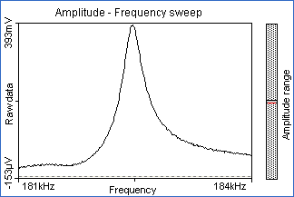
Frequency sweep of cantilever shows the resonance peak around 182 kHz.
When the tip contacts the surface, the high frequency 50 – 500 kHz makes the surfaces stiff (viscoelastic), and the tip-sample adhesion forces is greatly reduced. The dynamic mode inherently prevents the tip from sticking to the surface and causing damage during scanning. Unlike static mode, when the tip contacts the surface, it has sufficient oscillation amplitude to overcome the tip-sample adhesion forces. Also, the surface material is not pulled sideways by shear forces since the applied force is always vertical. Another advantage of the dynamic mode technique is its large, linear operating range. This makes the vertical feedback system highly stable, allowing routine reproducible sample measurements.
The dynamic operation in fluid has the same advantages as in the air or vacuum. However imaging in a fluid medium tends to damp the cantilever’s normal resonant frequency. In this case, the entire fluid cell can be oscillated to drive the cantilever into oscillation. This is different from the dynamic or non-contact operation in air or vacuum where the cantilever itself is oscillating. When an appropriate frequency is selected (usually in the range of 5,000 to 40,000 cycles per second), the amplitude of the cantilever will decrease when the tip begins to tap the sample, similar to dynamic mode operation in air. Alternatively, the very soft cantilevers can be used to get the good results in fluid. The spring constant is typically 0.1 N/m compared to the dynamic mode in air where the cantilever may be in the range of \(1-100\) N/m.
7.5.3 Force Curve Measurement
In addition to these topographic measurements, the AFM can also provide other data. The AFM can record the amount of force felt by the cantilever as the probe tip is brought close to - and even indented into - a sample surface and then pulled away. This technique can be used to measure the long range attractive or repulsive forces between the probe tip and the sample surface, elucidating local chemical and mechanical properties like adhesion and elasticity, and even thickness of adsorbed molecular layers or bond rupture lengths.
Force curves (force-versus-distance curve) typically show the deflection of the free end of the AFM cantilever as the fixed end of the cantilever is brought vertically towards and then away from the sample surface. Experimentally, this is done by applying a triangle-wave voltage pattern to the electrodes for the z-axis scanner. This causes the scanner to expand and then contract in the vertical direction, generating relative motion between the cantilever and sample. The deflection of the free end of the cantilever is measured and plotted at many points as the z-axis scanner extends the cantilever towards the surface and then retracts it again. By controlling the amplitude and frequency of the triangle-wave voltage pattern, the researcher can vary the distance and speed that the AFM cantilever tip travels during the force measurement.
Similar measurements can be made with oscillating probe systems like dynamic and *non-contact AFM}. This sort of work is just beginning for oscillating probe systems, but measurements of cantilever amplitude and/or phase versus separation can provide more information about the details of magnetic and electric fields over surfaces and also provide information about viscoelastic properties of sample surfaces.
Several steps of the force curve as shown in Fig.~\(\ref{fig:ForceCurve}\)
The cantilever starts not touching the surface. In this region, if the cantilever feels a long-range attractive (or repulsive) force it will deflect downwards (or upwards) before making contact with the surface.
As the probe tip is brought very close to the surface, it may jump into contact if it feels sufficient attractive force from the sample.
Once the tip is in contact with the surface, cantilever deflection will increase as the fixed end of the cantilever is brought closer to the sample. If the cantilever is sufficiently stiff, the probe tip may indent into the surface at this point. In this case, the slope or shape of the contact part of the force curve can provide information about the elasticity of the sample surface.
After loading the cantilever to a desired force value, the process is reversed. As the cantilever is withdrawn, adhesion or bonds formed during contact with the surface may cause the cantilever to adhere to the sample some distance past the initial contact point on the approach curve (B).
A key measurement of the AFM force curve is the point at which the adhesion is broken and the cantilever comes free from the surface. This can be used to measure the rupture force required to break the bond or adhesion.
One of the first uses of force measurements was to improve the quality of AFM images by monitoring and minimizing the attractive forces between the tip and sample. Force measurements were also used to demonstrate similarly reduced capillary forces for samples in vacuum and in reduced humidity environments.
7.5.4 Small Forces
Concern with the fundamental interactions between surfaces extends across physics, chemistry, materials science and a variety of other disciplines. With a force sensitivity on the order of a \(10^{-12}\) N, AFMs are excellent tools for probing these fundamental force interactions. Force measurements in water revealed the benefits of AFM imaging in this environment due to the lower tip-sample forces.
The liquid environment has become an important stage for fundamental force measurement because researchers can control many of the details of the probe surface force interaction by adjusting properties of the liquid. Experimentally, the electrostatic tip-sample forces depend strongly on pH and salt concentration. In fact, it is often possible to adjust the pH or salt concentration such that the attractive Van der Waals forces are effectively negated by repulsive electrostatic forces. This has been an important discovery because it can allow tuning of the liquid environment to minimize adhesive tip-sample forces that can damage the sample during imaging.
Atomic Force Microscopy has made its mark on a wide variety of applications as a topographic measurement and mapping tool. Now AFM force measurements are providing information on atomic- and molecular-scale interactions as well as nano-scale adhesive and elastic response. These measurements are beginning to revolutionize the way we quantitatively observe and, indeed, think about our chemical, biological and physical world.
7.6 Spike Tips
In contact AFM electrostatic and/or surface tension forces from the adsorbed gas layer pull the scanning tip toward the surface. It can damage samples and distort image data. Therefore, static mode imaging is heavily influenced by frictional and adhesive forces compared to non-contact or dynamic mode. With the dynamic mode technique, the very soft and fragile samples can be imaged successfully. Also, incorporated with Phase Imaging, the dynamic mode AFM can be used to analyze the components of the membrane.
If you run in dynamic mode, then it is necessary to find the resonance frequency of the oscillator first. In the dynamic mode the response is proportional to the derivative of the force \(F\).
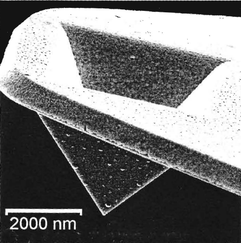
A scanning electron microscope image of a silicon nitride tip shows the pyramid at the end of the cantilever that is used for scanning.
The shape of the tip is very important in particular for magnetic force microscopy (MFM), where a magnetic coating is added to the tip. In that case the MFM tip may act as a magnetic dipole to detect the magnetic interaction forces.

A spike tip has been grown in a scanning electron microscope by using carbon impurities in the vacuum and focusing them to the end of the AFM tip. The spike tip is from \(300-600\) nm long and can be coated with Cr/Co for high-resolution MFM spectroscopy. Image: T.Gredig, M.S. Thesis (1998).
7.7 PID Parameters
The feedback loop in the AFM is controlled with proportional-integral-derivative (PID) parameters. This is a widely used method to control signals. In the case of AFM, the amplitude \(A(t)\) of the cantilever needs to be stabilized. The goal is to have \(A(t) = A_0\) (constant) by adjusting the height position. We will compute the error signal \(e(t)\), which is the difference between \(A(t)\) and the desired constant amplitude \(A_0\), or \(e(t) = A(t) - A_0\). The height signal \(\Delta h(t)\) to the piezo is now calculated as follows:
\[\begin{equation} \Delta h(t) = P e(t) + I \int*0^t e(t) \; d\tau - D \left( \frac{d}{dt} e(t) \right) \end{equation}\]
In electronics, the \(P\) value could be the resistor, the \(I\) corresponds to a capacitor, and \(D\) is the inductor. The proportional gain \(P\) allows to control how fast \(A_0\) is approached; the integral would dampen the overshoot, but if the oscillations around the set point \(A_0\) are too strong, then the derivative \(D\) factor ought be increased for under damping.
7.8 AFM Image Processing
There are several programs available for image processing of AFM images, see Table~??. Care must be taken, when loading the image, since one file can contain several images based on the recorded channels. For example, there could be one image showing the height and another showing the amplitude. The height image refers to the recording of the z-component of the piezo element, whereas the amplitude image is the rms amplitude of the cantilever. Strictly speaking in constant amplitude mode, the amplitude should be constant. Realistically, it contains the error signal of the z-component. Given the finite raster speed, the piezo element cannot respond quickly enough to keep the amplitude constant. Adjustments of the PID parameters, scan size, and scan speed can reduce the the contrast in the amplitude image, meaning that the cantilever tracks the surface more effectively. The quantitative analysis of the data requires careful calibration. The hysteretic effects of the piezo-element can even cause non-linear effects in the topography and overtime, the machine will get out of tune. Secondly, the image is always a convolution of the tip and the imaged surface, in particular for small scan sizes less than \(\approx\) 2\(\mu\)m.
As a first step, the image is “flattened”. In this part of the image processing the background slope is removed. It obfuscates the contrast of the image. Even though it appears that the sample was flat with respect to the surface, at the scale of nanometers, there always exists a tilt. This tilt is removed by subtracting a linear slope from the image. Once, the image is “flattened”, several parameters can be analyzed. This includes the surface roughness, the height difference between the lowest and highest point.
| Name | OS | WebSite |
|---|---|---|
| R | Mac, Windows | Gredig NanoscopeAFM |
| WSxM | Windows | WSxMsolutions.com, Ref. (Horcas et al. 2007) |
| Gwyddion | Mac, Windows | Gwyddion.net |
| Image SXM | Mac, Windows | ImageSXM.org.uk |
| GSXM | Ref. (Zahl et al. 2010) (Zahl et al. 2003) | |
| EasyScan | Windows | NanoSurf.com |
Using open-source software, we first install R Project for Statistical Computing, followed by the RStudio GUI. After launching RStudio, you can open and analyze AFM images using the Gredig nanoscopeAFM package. The latter package can be installed as follows:
install.packages(“devtools”) devtools::install_github(“thomasgredig/nanoscopeAFM”)
Once installed, you can import AFM data with AFM.import() and the use the plot() function to graph the image. Examples and descriptions of all AFM functions are documented.
library(nanoscopeAFM)
fileAFM = AFM.getSampleImages(type='ibw')[1]
d = AFM.import(fileAFM)
plot(d)
## Graphing: HeightRetrace
print(d)## Object: Cypher AFM Image
## Description: KC200, FePc, KC20170720Si
## Channel: HeightRetrace AmplitudeRetrace PhaseRetrace ZSensorRetrace
## 4000 nm x 4000 nm
## History:
## Filename: /Library/Frameworks/R.framework/Versions/4.2-arm64/Resources/library/nanoscopeAFM/extdata/AR_20211011.ibwsummary(d)## objectect description resolution size
## 1 Cypher Image KC200, FePc, KC20170720Si 128 x 128 4000 x 4000 nm
## 2 Cypher Image KC200, FePc, KC20170720Si 128 x 128 4000 x 4000 nm
## 3 Cypher Image KC200, FePc, KC20170720Si 128 x 128 4000 x 4000 nm
## 4 Cypher Image KC200, FePc, KC20170720Si 128 x 128 4000 x 4000 nm
## channel history z.min z.max z.units
## 1 HeightRetrace -32.5 50.8 nm
## 2 AmplitudeRetrace 29.0 32.8 nm
## 3 PhaseRetrace 63.9 85.2 deg
## 4 ZSensorRetrace -29.4 48.2 nm7.9 Height-Height Correlations
Images often contain small particles, the distribution and particle size is generally of interest. The particle size can be determined from the correlation function. In particular, the height-height correlation function \(h(r)\) is defined as
\[\begin{equation} h(r) = < | h(\vec{r}_1) - h(\vec{r}_2)|^2 > \end{equation}\]
the average square of the height difference between two points that are located at position \(\vec{r}_1\) and \(\vec{r}_2\). The distance between these two points is \(r\). Immediately, it follows from the definition that $h(0) = $ 0 nm2. Secondly, for large distances, as it approaches the image size \(a\), the function measures the long-range roughness, \(lim_{r \rightarrow a} h(r) = 2\sigma^2\), where \(\sigma\) is the rms roughness of the image. Empirically, it has been observed that \(h(r)\) closely follows
\[\begin{equation} g(r) = 2\sigma^2 \left[ 1 - \exp{ \left[- \left( \frac{x}{\xi} \right)^{2 \alpha} \right]} \right] \tag{7.5} \end{equation}\]
where \(\xi\) is the correlation length, which is proportional to the average particle size, and \(\alpha\) is the Hurst factor, which measures the short-range roughness. This parameter should be in the range of 0.5 to 1.0 (Gredig, Silverstein, and Byrne 2013).
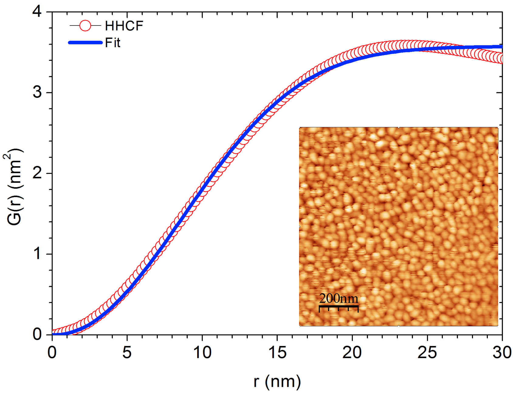
The inset shows an AFM image of a thin film of phthalocyanine molecules. The molecules form small grains. The height-height correlation function is computed and fit to Eq.@(eq:hhcf) for comparison.
7.10 Problems
Using the Lennard-Jones potential, (a) graph the energy for argon gas and find the equilibrium position \(d_0\), (b) find a general expression for \(d_0\) given \(A\) and \(B\) constants.
Calculate the spring constant \(k\) of a diving board with length 5m and width 1m and thickness of 1 cm.
Find the dimensions for the commercial Aspire CT170 tip to compute its resonance frequency \(\omega_0\) and compare with the provided values.
Compare the cantilever motion, a forced damped harmonic cantilever, with a battery powered LRC circuit. How are the inductance, resistance, and capacitance related to the spring constant, mass, and Q factor?
Given the resonance curve in Fig.~??, find the Q-value of the cantilever.
Graph Eq. (7.2) for the three regimes of \(\beta\).
What is the Q-factor for your tip (you can measure it)? Which kind of tip did you use and what is the resonance frequency?