Lab 1 Uncertainties
The physical sciences are based on real-based measurements. Measurements come with a certain accuracy and precision. It is important to distinguish these terms and use them correctly in the lab notebook reports. Repeated measurements and successive refinements lead to gradually more reliable description of events and improvement of precision.
By the end of this activity, you should be able to do:
- Understand assumptions, limitations, and uncertainties of an experiment (Modeling);
- Use precision measurement tools to accurately measure quantities including their uncertainties (Practical Skills);
- Able to propagate uncertainties (Analysis);
- Share and state data with significant digits and uncertainties (Communication Skills).
1.1 Introduction
1.1.1 Accuracy and Error
An error in science generally refers to the difference between the measurement \(x\) and the actual value \(A\) (or known value). Often times, the known value is not known. If it is, however, the error can be computed. It is a positive value. It is also useful to discuss the relative error measured as a percentage. The relative error \(RE\) is:
\(RE = 100 \frac{| x - A | }{A}\)
The error reflects the accuracy of the measurement. It is a good quantity to include in your summary.
Example: There are 152 apples on a tree. Since the average apple weighs 0.05 kg, and the total amount of apples is 7.5 kg, your measurement indicates that there are 150 apples. That means that the error is 2 apples, or the relative error is 1.3%.
1.1.2 Uncertainty
Uncertainty and significant figures (or significant digits) are distinct quantities from the error discussed earlier. Each measurement is limited by the measurement device to a specific precision. Using a stop watch, you may measure the time for a ball to roll a specific distance downhill. Repeating the measurement several times will give you several different results. This “random error” due to the variability is called the uncertainty. In this case, the reaction time may be important. Additionally, the time spacings of the stop watch limit the precision. It could be a stop watch with second resolution, or another stop watch that has 1/100 second resolution. Similarly, the distance can have an uncertainty due to the meter stick used.
In the example of shooting arrows at a center target (bull’s eye), precise but not accurate would mean that all the arrows are close to each other, but not in the center. If the arrows are spread around the center, it would be accurate, but maybe not precise, since the arrows are spread far from the center. If all arrows are exactly in the center, then they are both accurate and precise. You can reduce the precision by making more observations or changes to the measurement procedure.
1.1.3 Significant Digits
When reporting numbers in the epxerimental laboratory, the correct number of significant digits must be included and is determined by the uncertainty of the measurement. Each number \(x\) can be expressed with a significand \(m\) and exponent \(n\), as \(x = m \cdot 10^n\), where \(n\) is an integer. As an example, 150 could be \(1.5 \cdot 10^2\). The number of digits of the significand are called significant digits. The number 134 has 3 significant digits, and 23.44 has 4 significant digits, whereas 0.00041 has only 2 significant digits. The number 150 is ambiguous, since it could have 3 or 2 significant figures; therefore, it is best to write \(1.5 \cdot 10^2\) or \(1.50 \cdot 10^2\) in order to make the distinction. From an experimental point of view, the numbers 4 and 4.0 are different.
For this lab, the uncertainty has always 1 significant digit, so \(\Delta x = 0.02\) m, for example. You could express your height as \((1.61 \pm 0.02)\)m.
1.1.4 Uncertainty Measurement
Each time something is measured with an instrument (ruler, digital multimeter, stop watch), you will need to also record the resolution or uncertainty of the measurement. Next, when you compute a resulte, you will need to propagate the uncertainty.
The uncertainty may be reduced, if you make repeated mesurements, this is called the statistical uncertainty.
1.1.5 Resolution (uncertainty measurement)
The first rule is that the uncertainty is no smaller than half the smallest spacing. So, 0.5 s is the “best” or smallest uncertainty for the stop watch with one second resolution, and 0.5 mm for the ruler with 1 mm spacings.
For example, if you are using a ruler with markings every 1 mm, then your accuracy is 0.5 mm or half the smallest division. This is called the resolution.
1.1.6 Statistical Uncertainty
If you have many measurements, \(x_1, x_2, \ldots, x_N\) then mean value \(\bar{x}\) is calculated (or use =AVERAGE() function in a digital spreadsheet):
\(\bar{x} = \frac{1}{N} \sum_{i=1}^{N} x_i\)
and the standard deviation would be \(\Delta x\) calculated as (or use =STDEV() function in a digital spreadsheet):
\(\Delta x = \sqrt{\frac{1}{N-1} \sum_{i=1}^{N} (x_i -\bar{x})^2 }\)
For practical reasons, in the introductory laboratory, you may use the emperical uncertainty calculation: if you make less than 10 measurements, then use the mid-point of all measurements as the measurement value \(x\); ergo, find the largest value \(x_{max}\) and the smallest measurement value \(x_{min}\), then
\(\bar{x} = \frac{1}{2} (x_{max} + x_{min})\)
The uncertainty \(\Delta x\) is the half-width of the measurement range, so
\(\Delta x = \frac{1}{2} (x_{max} - x_{min})\)
Your results are expressed as \(\bar{x} \pm \Delta x\). The second rule is that \(\Delta x\) has only 1 significant digit, so that you then adjust \(\bar{x}\) with the appropriate number of significant digits.
Example: You measure the thickness of a book with a ruler that has 1 mm divisions 4 times: 2.2cm, 2.5cm, 2.4cm, and 2.1cm. This book is \(2.3 \pm 0.2\)cm thick. Another book was measured: 2.2cm, 2.2cm, 2.2cm, and 2.2cm. Thus, the thickness is \(2.20 \pm 0.05\) cm, since the measurement is limited by the ruler in this case. In the former case, the relative uncertainty is 9% and in the latter case it is 2%.
1.1.7 Propagation of Uncertainty
Often you make several measurements to find a result; i.e. to measure speed, you would measure distance and time. Each separate measurement has an uncertainty, so how would you combine them and report the uncertainty of the final result; i.e. the speed?
Your experimental uncertainty is very important, so two methods are presented to deal with this.
- Emperical propagation method using worst case scenario
- Common formula for indepdent variables
In the emperical propagation method, you calculate the worst case scenarios and compute the difference from the average result, so propagate the uncertainty by re-computing the value, if you were measuring different numbers using the uncertainty. If you mulitply, you would use the \((x + \Delta x)\) and if you divide \((x - \Delta x)\), since a number gets larger, if you divide by a smaller number, see second example.
Example: Given an relation of area = length x width, then \(A = l w\), and the length is mesured as \(l \pm \Delta l\) and the width \(w \pm \Delta w\). The \(A_{max} = (l+\Delta l)(w+\Delta w)\), and the uncertainty \(\Delta A = A_{max} - A = w \Delta l + l \Delta w + \Delta w \Delta l\).
Example: of a toy car that traverses a distance \(d = 15 \pm 1\)cm in time \(t = 2.3 \pm 0.1\)s, the speed would be \(v=d/t\), so \(v\)=6.52 cm/s. The worst case for high speed would be a longer distance 16cm and a shorter time of 2.2s, both values lie within the measurement uncertainty. We would obtain \(v\)=7.27cm/s. Therefore, \(\Delta v\) = 0.75cm/s. Using the opposites of 14cm and 2.4s, \(v\)=5.83cm/s, off by 0.68 cm/s.
According to rule 2, there is only one significant digit, so \(\Delta v\)=0.8cm/s and the final result is that the toy car has a measured speed of \(6.5 \pm 0.8\) cm/s.
The Jacobian propagation method is simply given by this common formula for independent variables. A function \(f\) with variables \(x_i\) that each have uncertainties \(\Delta x_i\) would be computed as:
\(\Delta f \simeq \sqrt{ \left( \frac{\partial f}{\partial x_1}\right)^2 (\Delta x_1) ^2 +\left( \frac{\partial f}{\partial x_2}\right)^2 (\Delta x_2) ^2 + \ldots }\)
Hence, for the example where \(f=v\), and \(x_1=d, x_2 = t\), we find that
\(\Delta v = \sqrt{ \frac{(\Delta d)^2}{ t ^2} + \frac{d^2}{t^4}(\Delta t)^2}\)
easily transformed in an expression with relative errors
\(\Delta v = v \sqrt{ \left(\frac{\Delta d}{d}\right)^2 + \left( \frac{\Delta t}{t} \right)^2}\)
which yields \(\Delta v=\) 0.5 cm/s. The uncertainty is a bit smaller, since it takes into account that the both extremes are unlikely to occur, we find: \(v = 6.5 \pm 0.5\) cm/s, which can be interpreted that if measured again under the same conditions, the result would fall in this range with 67% chance (see RC Lab).
1.1.8 Weighted Average
In the case that two teams make the same measurement, the two results can be combined commonly in a weighted fashion. Under many circumstances, the weight \(w_i\) can be estimated to be
\(w_i = \frac{1}{(\Delta x_i)^2}\)
where \(\Delta x_i\) is the uncertainty of a measurement. The averaged value would be
\(\bar{x} = \frac{\sum_i w_i x_i}{\sum_i w_i}\)
Example: The diameter of tennis balls are measured and team 1 finds (\(11 \pm 1\)) cm, while team 2 finds (\(10 \pm 2)\) cm. The weight of team 1’s ball would be \(w_1 = 0.8\) and then the so computed weighted diameter would be (\(10.8 \pm 0.9\)) cm.
1.1.9 Systematic Errors
Additionally, there can be systematic errors. These refer to un-calibrated devices. As an example: a scale shows 3g without load. It would be systematically off by 3g for each measurement. In another example, you measure the distance between a compass and a point. Instead of measuring from the center of the compass, you measured from the edge, so your measurements may be systematically off by a certain distance.
1.1.10 Instruments: Caliper
Rulers are used to measure length, but to get more precision, a caliper can be used. The caliper consists of two parts, which can move relative to each other. In addition to the regular ruler scale in units of mm, it has a Vernier scale that usually has a resolution of 0.05 mm or as noted on the specific caliper. The thickness of a book may be read of as 2.1x cm, where \(x\) represents the unkown digit. The Vernier scale has 10 additional steps that need to be visually aligned. From the 10 lines, only one matches exactly the top line. The line number provides the unkown \(x\) digit. For example, if the forth line matches, then the book thickness would be 2.14 cm.
1.2 Goals
- Measure the area and volume of a piece of paper;
- Practice to measure and propagate uncertainties;
- Learn to use a scientific instrument, the caliper;
- Realize that there are several ways to measure the thickness.
- Attempt to make the most precise measurement possible.
- Find out how much each parameter (length, thickness, width) contributes to the uncertainty of the volume.
1.3 Prediction
- Write an equation for the area and volume of a piece of paper. Draw a schematic.
- Use quick estimates (basic assumptions) to find an approximate value for the total area and volume of a piece of paper (without completing the measurement). Express in units of cm\(^3\).
- How could you improve the precision of the thickness measurement?
1.4 Equipment
- 3 pieces of paper
- Ruler (metric) and caliper
- Calculator
1.5 Procedure
- Use a ruler to determine the length and width of a piece of paper. Every team member should make at least one indepedent measurement and report with their uncertainty. Then combine the individual results.
- Determine the thickness of a piece of paper using a caliper and varying the number of layers. Record your results in a table and compute the thickness of one layer with its uncertainty Note that the uncertainty only has 1 significant digit precision.
- Compute the volume of a piece of paper and propagate the uncertainty.
- Check that the results are reasonable and how they agree with the predictions, then repeat and reduce the uncertainty by making more careful measurements or using a different approach based on what you have learned.
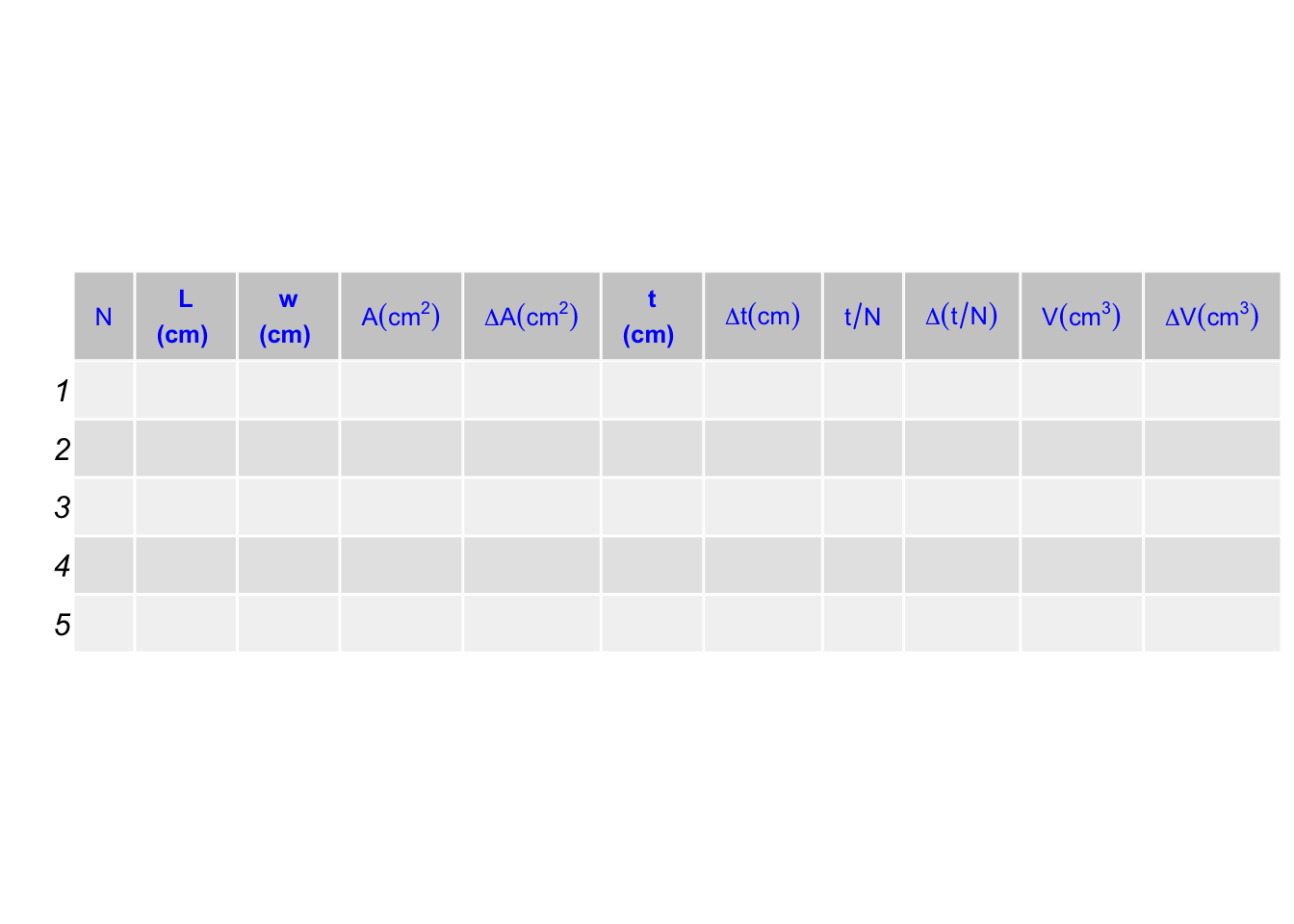
1.6 Table
Create a table with useful quantities that you measure. It can look similar to the one below, but may include additional or different columns, such as \(\Delta w\). The column headers refer back to the schematic diagram that you have. For illustration, we choose N = number of stacked paper layers, L = length, w = width, t = total thickness, A = area, V = volume per layer. Also, \(\Delta t\) and \(\Delta V\) are the uncertainties for thickness and volume. You may use several tables instead. Use different ways to determine the thickness of the sheet of paper and list each result. Which method is the most precise and what is the best uncertainty that you can find reliably.
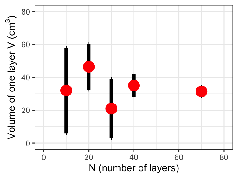
1.7 Graph
Make a graph of the volume (V), which is the dependent variable versus number of layers (N), which is the independent variable, and include the uncertainty in the diagram. Other graphs are also possible as long as the x-axis has the independent variable. Always use a ruler and label the axes. What can you learn from the results? Note your observations in the lab notebook.
1.8 Discussion
Share the thickness \(t\) per layer and the best uncertainty \(\Delta t\) that you found for one layer. Report the volume \(V\) and its uncertainty \(\Delta V\). Discuss the best method to measure the paper thickness precisely. Discuss any problems that occured.
1.9 Summary
Your summary should answer the questions set forth in the goal section. Include the one quantitative results that represents the main finding. Also, include information such as the precision of the ruler and the precision of the caliper. Discuss how you went about to make the most precise measurement possible and list both your findings of the volume \(V\) with the uncertainty, in addition to the findings from the class. Compare your results with the measurements from other groups in your class.
1.10 Additional Reading
Philip R. Bevington and D. Keith Robinson, Data Reduction and Error Analysis for the Physical Sciences, 2d Edition, WCB/McGraw-Hill, 1992
Accuracy and Precision: https://labwrite.ncsu.edu/Experimental%20Design/accuracyprecision.htm
Measurements and Significant Digits: http://www.ligo.caltech.edu/~vsanni/ph3/SignificantFiguresAndMeasurements/SignificantFiguresAndMeasurements.pdf
Calipers: https://en.wikipedia.org/wiki/Calipers
Paper Thickness: https://www.printi.com/blog/thickness-of-paper/
Dependent and Independent Variables: https://mathbench.umd.edu/modules/visualization_graph/page02.htm