Lab 6 Electric Potential of Dipole
Electric fields describe the electric potential or electric “landscape”. The electric field vector has both a direction and magnitude. However, it will be easier to measure a scalar quantity, which is the electric potential. The definition of the electric potential is \(\Delta V = -\int (E_x dx + E_y dy + E_z dz)\). It represents the voltage between two points and it is analogous to a height difference or altitude (with respect to sea level). The electric field is analogue to acceleration, or pouring water and watching in what direction it flows, if it is steep it will flow quickly downwards, if the slope is small, it will flow slowly. The speed corresponds to the magnitude. The Digital Multimeter can measure the electric potential between two points, the “height difference” between two points. By measuring the electric potential at sufficiently many points, you can map the “height” profile and then create the electric vector field it results from. In particular, you find the slope or magnitude of the electric field, by measuring the electric potential at two close points, then \(|E| = \Delta V / \Delta s\), where \(\Delta s\) is a “short” separation distance. By connecting locations with the same potential, you create equipotential lines, the direction of the electric field is perpendicular to the equipotential line. Note that the units of the electric field: (N/C) can also be written as (V/m).
6.1 Goals
- Measure the electric vector in several locations
- Find two locations, where the magnitude of the electric field vector is different by a factor of 10.
- Measure the electric potential \(\Delta V\) across capacitor plates
6.2 Prediction
- Draw two parallel electrode bars and add five positive charges uniformly distributed in one of them, add five negative charges in the other. Given those charges, draw the electric field vector at positions between the bars, above, and outside the bars.
- Draw a line perpendicular to the bars, crossing both at the center, similar to the Figure. Then make a graph of the electric potential \(\Delta V\) as a function of the position \(x\).
- Mark two places on the diagram, where the electric field is different by a factor of 10.
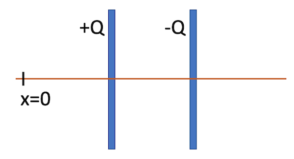
Charged capacitor plates with a measurement line crossing them. Measure the electric potential along this line.
6.3 Equipment
- Digital Multimeter
- Power supply (run between 1 and 3 V), record the exact value!
- Carbon paper (conductive) (keep scratch-free)
- Copper electrode bars (2x)
6.3.1 Caution
- Avoid scratching the surface of the carbon paper by not dragging the tool on the surface.
6.4 Procedure
Connect two banana wires from the power supply to the electrode bars mounted on the carbon paper to create a circuit.
Connect the ground wire from the multimeter to the ground plug on the power supply.
Connect the multimeter to measure the electric potential difference across the two plates by touching the second plate. Adjust the voltage until you have something between 1 and 3 V. Record the value.
Learn how to use the digital multimeter, explore all buttons and discuss with team.
Since the carbon paper is conductive, you can connect to different locations on the board and record the voltage difference. Do not move the electrode, lift it to move it to a new location.
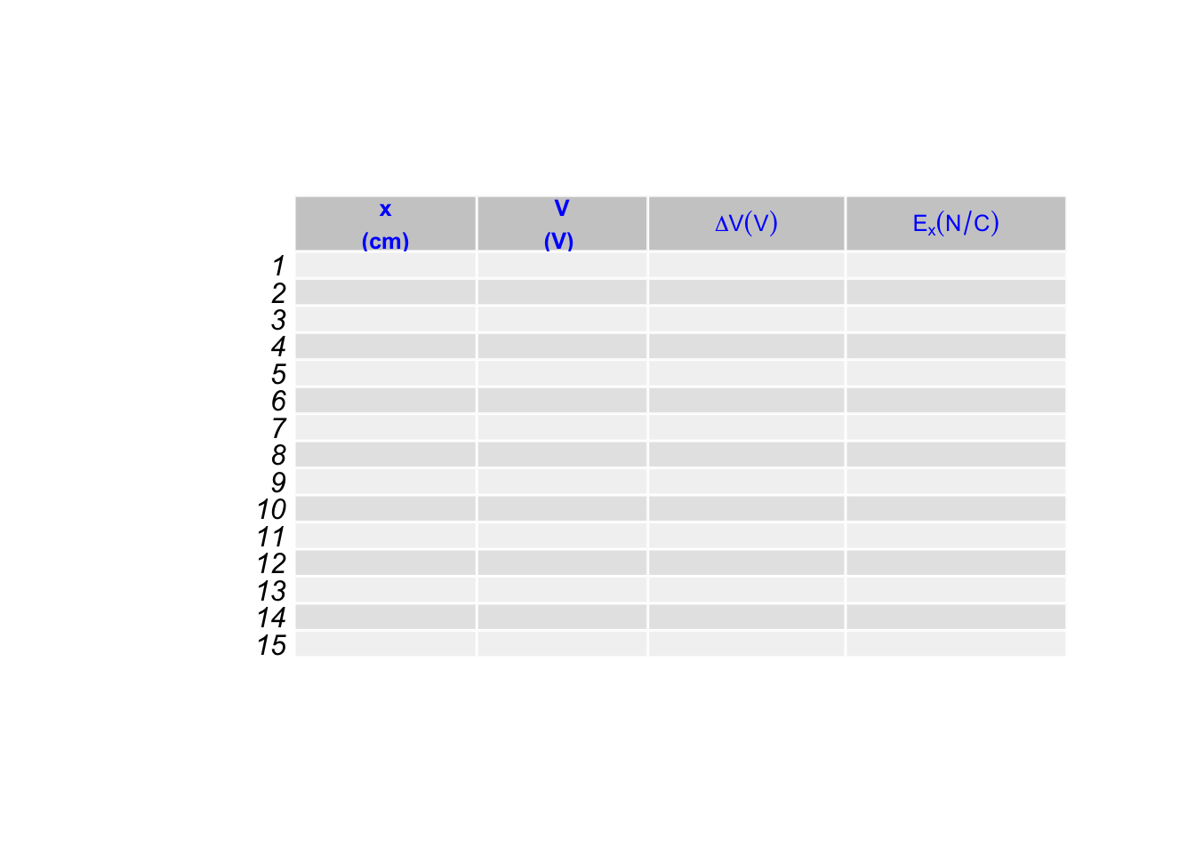
Measure the electric potential at about 20 points along the axes that crosses both electrodes. Make sure to have data points both far away from the electrodes as well as nearby and between the electrodes.
Measure the electric field at one location between the electrodes. Choose two nearby points along the x-direction and measure the potential difference, then repeat for the y-direction at the same location to determine \(E_x\) and \(E_y\) separately. You will need both components to calculate the magnitude of the electric field \(|\vec{E}| = \sqrt{E_x^2 + E_y^2}\).
Guided by your predictions, find two locations where the electric field varies by a factor of 10.
6.5 Measurement
Create a table similar to this one; it should contain at the minimum 20 data points and cover the distance from the ends of the carbon paper. In interesting regions take more data.
6.6 Graph
Make a graph of the electric potential \(\Delta V\) as a function of the position \(x\) across the capacitor plates and compare with your predictions. Make sure to clearly label the positions of the electrode edges and the carbon paper edges on your graph.
6.7 Discussion
Compare your graph of Electric Potential versus distance with the predictions. Share the graph with the class, include quantitative scales. What does the shape tell you? What can you tell about the electric field from the graph? Where is the electric field the strongest?
6.8 Summary
Discuss the goals. Make sense of the predictions and measurements. Mention the coordinates of the two points that have electric field magnitudes, which are 10x different, include their values. In the reflections: What are you surprised about?