GEOG 140 Chi-Squared Lab: Dr. Rodrigue

Geography 140

Introduction to Physical Geography

Lab 6: Introduction to Statistical Hypothesis Testing

==========

This lab covers a useful technique for hypothesis-testing, using spatial data in biogeography. It is called "Chi-squared" (pronounced "Kye" to rhyme with "eye"), and here we'll use it in quadrat analysis or analysis of data from a grid. Chi-squared is sometimes

Background on Statistics

Statistics can be divided into two main areas of concern. One is simply the description of a population or sample taken from that population. Descriptive statistics include such things as measures of central tendency (such as means or averages and medians or middle scores), measures of variability (such as the range from high score to low score or the standard deviation), and measures of a distribution's shape (such as skewness). You're probably already pretty familiar with these, if for no other reason than that professors often share with you some of these measures for their classes. Inferential statistics is the other big concern of statistics and one of the reasons it is so powerful and influential. It involves making inferences about the characteristics of a population from a study of a smaller sample. It is one of the most common methods used in all of the sciences, from the natural sciences (including physical geography, geology, astronomy, and biology) to the social sciences (including human geography, sociology, economics, political science, psychology, and anthropology). In fact, it is really common in business, too (especially marketing) and is critical in engineering, too (figuring out likelihood of a bridge collapsing).

So, "building character" in this lab will pay dividends for you in all kinds of pursuits, no matter your major and eventual job. Chi-squared is one of the very simplest inferential statistical tests you can do, and it is very flexible in terms of the kinds of data you can use it to analyze: All you need to do is set up your data as frequency counts (nominal level data).

In fact, if you get the hang of Chi-squared and can apply it appropriately in term projects in other classes, you will almost certainly really impress your other professors ;-) -- and with relatively little effort! How's that for a dividend?

For all questions on this lab, please do your calculations at the full capacity of your spreadsheet or calculator (don't round at each step), but round your answers at the end to two decimal places of accuracy (i.e., 0.00).

Chi-Squared Quadrat Analysis

Quadrat-based techniques of spatial, geographical analysis involve the division of a study area into equal-sized plots, called "quadrats," usually through a grid of squares. This permits fairly easy data collection, just counting occurrences by quadrats.

By using quadrats to sample data in a region, we have moved into the area of inferential statistics. Inferential statistics lets us characterize a population (the larger region) through data drawn from a smaller sample. The reason we would want to do this is it takes less time and money to study a sample than to try to take on the whole population.

Inferential statistical analysis lets us decide whether pure random selection could have created a sample as extremely different from expectation as the one we wound up with. In other words, we can decide, in this case, whether two factors are positively associated together or negatively associated.

Now, there is always the small chance that pure random chance can create the illusion of association. The neat thing about inferential statistics is that we can actually give the probability that our answer is wrong. Hunh? This may make a bit more sense after going through the lab assignment.

For your reference pleasure, the definitional formula for Chi-squared is:

          r   k                       
         __  __  (O_ij - E_ij)²
     X² =\   \  ____________
         /_  /_      E_ij
         i=1 j=1

You'll be comforted to know I'll walk you through a much easier computational process. Had you going there, I'll bet.

About the Case Study

In this lab, you are looking at two plant species that both occur in a study area in Southern California. One is Salvia apiana or white sage (a native California shrub), and the other is Avena barbata or slender oat (an introduced exotic grass originally from the Mediterranean). The grass tends to be invasive, but the sage is not without ability to protect its turf from grass seedlings. They are often found in the same general region but the close up geography may not accord with that impression. Scale is important to geographers! Here are pictures:

Lab 6a: Setting up Hypotheses

The first order of business is to set up your working hypothesis. So, eyeballing the map in Figure 1, formulate your hunch about the association between the two plant species described below at the scale of the map. Do they hang out together (a positive association) or do they repel one another (negative association)? Basically, at this point, decide whether they look like they're associated (positively or negatively). Your hunch is called the "working hypothesis." Please state your working hypothesis:
```
     _________________________________________________________________________

     _________________________________________________________________________

     _________________________________________________________________________

     _________________________________________________________________________
```
In statistics, it violates logic to think that you can directly prove this hypothesis (or any other one in science). To think that, because results square with your expectation, you have "proven" that one thing accounts for another is a logical fallacy called "affirming the consequent" (which means that you're overlooking the possibility that some other factor you never even imagined might explain your results). Some of the reasoning behind this came up earlier in the online lecture about the nature of science at https://home.csulb.edu/~rodrigue/geog140/lectures/science.html.
All you can do in science (or statistics) is disprove various alternatives. So, our second order of business is to set up a null hypothesis, which is the opposite of your original working hypothesis. That is, if you suspect that A and B are significantly related somehow (your working hypothesis), your null hypothesis would be "there is no significant association between A and B." Then, if you disprove the null hypothesis, your original working hypothesis comes out as the only viable alternative: You haven't proved it, mind you, but you have disproved its opposite. Got all that? Okay, what would your null hypothesis be, then?
```
     _________________________________________________________________________

     _________________________________________________________________________

     _________________________________________________________________________

     _________________________________________________________________________
```

Lab 6b: Setting up a Criterion to Judge Your Null Hypothesis ahead of Time

Our third order of business is to set an appropriate standard to judge whether the null hypothesis can be rejected for your purposes. This is called "alpha." Let's set our standard of judgment, or alpha, at the 0.05 level. You have to set alpha ahead of time, so you're not tempted to say, "sheesh, this just missed being significant, so I'll just SAY my alpha was whatever."
Hunh? This means that we will reject the null hypothesis only if the results are so extreme that there's less than a 5% chance that just random luck of the draw could have created a sample with such extreme characteristics. In other words, we'll reject the null hypothesis if it has less than a 5% chance of being true. This means that we feel better about our original hunch, with at least 95% confidence. If you were about to go out in the field yourself, you would want to think about where to set alpha to balance the risks of thinking you see a pattern when there really isn't one or of thinking nothing's going on when there really is. The 0.05 standard is very common in most sciences, by the way.

Lab 6c: Calculating X² from Your Observations

Classifiying and counting your observations are the next steps. Figure 1 mentioned above shows the distribution of two plant species, Salvia apiana (white sage) and Avena barbata (slender oat). Let's look at the map in a little more detail. Each of the larger quadrats (the ones labeled A1 or F9 or J5, for example) can be classified into one of the four quadrat types listed below
- (a) containing both Avena and Salvia;
- (b) containing Avena but no Salvia;
- (c) containing Salvia but no Avena; OR
- (d) containing neither Avena nor Salvia.
You will be relieved to know that it isn't going to be you out there counting and classifying and keeping track of 100 quadrats! The data are already shown in an answer sheet kind of like this one at https://home.csulb.edu/~rodrigue/geog140/labs/chisquarecounts.gif.
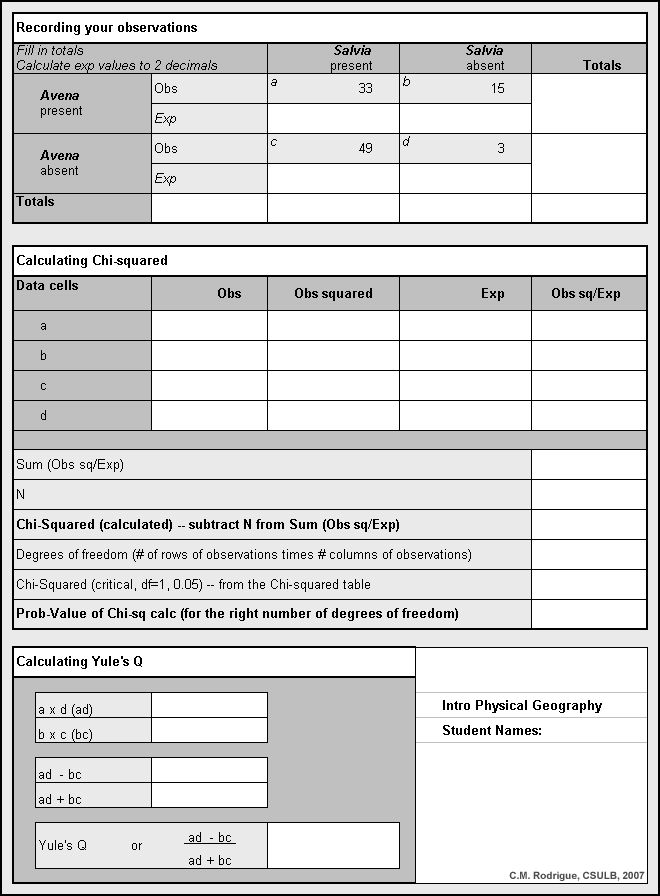
```
                      |                  SALVIA                 |
                      |                    |                    |
                      |      present       |       absent       |   row totals
     _________________________________________________________________________
                      |(a)                 |(b)                 |-e-
           present    |                    |                    |
                      |                    |                    |
     AVENA   _________________________________________________________________
                      |(c)                 |(d)                 |-f-
           absent     |                    |                    |
                      |                    |                    |
     _________________________________________________________________________
                      |-g-                 |-h-                 |-i-
     column totals    |                    |                    |   
                      |                    |                    | n = 
```
Now, it's your turn to do some work. Compute the "marginal totals." That is, sum the observed frequencies in each row and put those sums in the appropriate row total (corresponding to e or f in the sketch above). Do the same for the frequencies in each column and put those sums in the appropriate column total (corresponding to g or h here). The sum of row totals should equal the sum of column totals. If so, put the total number or n (which had better equal 100) in cell i.
Create the "expected frequencies" for each data cell (a through d). This is the distribution of cell counts you would expect from your data if there were no association between the two plant species (i.e., random processes were allocating them among the cells). To do this for each data cell, a through d, multiply the row total to its right by the column total below it and then divide the answer by n. Put the answer, rounded to two decimal places of accuracy, in its cell below the actual observed frequency.

Still lost? Okay, okay. In other words, multiply cells e and g and divide the answer by cell i. Put the answer, properly rounded, in the lower part of cell a. Similarly, multiply cells e and h and divide by i, and put that answer in cell b. Multiply cells f and g and divide by i, and plop that answer in cell c. Lastly, multiply cell f by cell h, divide by i again, and put the result in cell d.

That done, examine the expected frequencies. Chi-squared should not be used if any expected frequencies are below 2 (or, irrelevantly in this case, if more than 20 percent of the data cells have fewer than 5 actual cases). You will note that there are no such problems with your contingency table, so you can safely proceed through Chi-squared.
Now, move on to the worksheet below the data entry sheet for calculating Chi-squared. In the first column, enter the observed frequencies for each data cell (the number in the upper part of cells a through d).
In the second column, square those frequencies (that is, multiply each observed frequency by itself).
In the third column, divide each squared observed frequency by the corresponding expected frequency in the bottom of the appropriate data cell (a through d).
Now, sum up the third column and put the answer near the bottom of the worksheet (sum(O²/E). Show your work here to two decimal places of accuracy.

Finally, subtract n (which is found in cell i, the lower right corner of your data entry sheet) from that sum. This answer is your calculated Chi-squared (X²)! Put it at the bottom of the whole worksheet, also rounded to two decimal places of accuracy. Do this on the much more æsthetic answer sheet provided at https://home.csulb.edu/~rodrigue/geog140/labs/chisquarecounts.gif

     ________________________________________________________________________

     DATA CELL |     O     |       O²       |          O²/E
     ________________________________________________________________________
        (a)    |           |                |
     ________________________________________________________________________     
        (b)    |           |                |
     ________________________________________________________________________
        (c)    |           |                |
     ________________________________________________________________________
        (d)    |           |                |
     ________________________________________________________________________
                                            | sum(O²/E) = 
     ________________________________________________________________________
                           |         sum(O²/E) - n = X² =
     ________________________________________________________________________

Now, to interpret this hard-gained number, your X²_calc, you need to compare it with a critical X². To do this, you will need to consult a Chi-squared table, such as this one from the StatSoft online statistics textbook.
Getting into the table is a little tricky. You need your pre-selected alpha level to pick the right column and the degrees of freedom for your 2 row x 2 column contingency table to choose the right row to enter the table. Degrees of freedom in Chi-squared can be defined as:
```
     DF = (r - 1)(k - 1)
     where r = number of rows and k = number of columns 
               (you multiply the two subtractions' answers together)
```
So, you will enter the table at the intersection of:
```
     the column headed ________ 

     and the row corresponding to ________ degrees of freedom.
```
What, then, is your critical Chi-squared value?
```
     X²_crit =  ________
```
Now, you need to compare your X²_calc with the table's X²_crit. Is your X²_calc ________ greater than or ________ less than the X²_crit?
If your actual, calculated Chi-squared value is greater than the critical Chi-squared, you may safely conclude that your pattern is not just a random one. In other words, there is a statistically significant probability that there is a real association of some sort between your variables (in this case, between the two plant species). If the calculated Chi-squared value is less than the critical test value, the relationship probably is random. Can the null hypothesis of random association between these two plant species in this study area be rejected in this case?
```
     _____ reject H_o          _____ do not reject H_o
```
It's always good etiquette, whenever possible, to calculate the probability of making an error in rejecting the null hypothesis. This is called the "prob-value," and you can think of it as your belief in the pure randomness of your association. This extra courtesy step is done in the off chance that a reader may have compelling reasons to use a different standard of alpha than you chose. Consult https://home.csulb.edu/~rodrigue/geog140/labs/chisquareprobvalues.xls to get the probability (for one degree of freedom) that you could have gotten results as extreme as yours if there is really nothing but a random association between the two plant species.
```
     ________ prob-value of H_o
```

Lab 6d: Calculating Yules' Q to Assess the Strength of Association

Plot complication. Chi-squared is notoriously sensitive to sample size. That is, the same percentages in each cell can appear significant in a big sample (large n) or insignificant in a small sample. It might help to assess the strength of a significant relationship, should the Chi-squared test find one. For that, you can use "Yule's Q." Yule's Q, however, can only be calculated for contingency tables with no more than two rows and two columns (bigger tables can sometimes be collapsed into a 2 x 2 format, by combining rows and columns in some sort of logical way). Conveniently, this lab just happens to feature a 2 x 2 table.
To calculate Yule's Q, multiply cells a and d and also cells b and c. Then, enter these multiplications into the following formula:
ad - bc Q = _______ ad + bc
So, what is the Q value for this lab? ________
Now, what does it all mean? Basically, Yule's Q can vary from -1 to +1. The closer it is to 0, the weaker (more random) the relationship is. The closer it is to -1 or +1, the stronger the relationship is, whether inverse (negative) or direct (positive). So, what does the Yule's Q statistic look like to you in terms of direction and strength of association?
```
     _________________________________________________________________________
```

Lab 6e: Discussion and Write up

Please discuss and then individually write up your analysis of this lab, taking into consideration the results of both Chi-squared and Yule's Q. Is there a significant ecological association between Salvia apiana and Avena barbata at this scale of analysis? (results of your Chi-squared analysis). If so, what is the nature of that association (direct or inverse, which the sign of Yule's Q can tell you)? How strong is it (the value of Yule's Q)? In ordinary English, what is going on between these two species at this scale of analysis? What could be producing these results?
```
     _________________________________________________________________________

     _________________________________________________________________________

     _________________________________________________________________________

     _________________________________________________________________________

     _________________________________________________________________________

     _________________________________________________________________________
```

Figure 1

The map of oats and sage from which the data in https://home.csulb.edu/~rodrigue/geog140/labs/chisquarecounts.gif are taken. You can see why the Department doesn't let me teach cartography!