Back to Problems

Taylor Series Plots with Animation

Please Click on ANIMATION to see the Mathematica code for the above Taylor Series animation.

Taylor Series

H.Tahsiri

Off[General::spell];
Off[General::spell1];
Pagewidth->70;

f[x_]=Sin[x]

     Sin[x]

(* Taylor polynomal of order n=9 near point a=0 *)

1) Generate a polynomial of 10 element

Table[poly[x_,n]=Series[f[x],{x,0,n}]//Normal,{n,0,9}];

2) generate p1,p2,p3 and p9 of order n=1,2,3 and 9

p1=poly[x,1] (* Taylor polynomial of order n=1 *)


     x

p2=poly[x,5] (* Taylor polynomial of order n=5 *)


          3    5
         x    x
     x - -- + ---
         6    120

p3=poly[x,3] (* Taylor polynomial of order n=3 *)


          3
         x
     x - --
         6

p9=poly[x,9] (* Taylor polynomial of order n=9 *)

          3    5      7       9
         x    x      x       x
     x - -- + --- - ---- + ------
         6    120   5040   362880

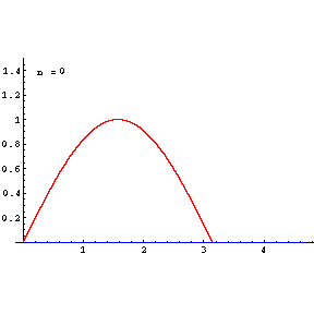
3) Plot of y(x)=f(x)=sin(x)

plotf=Plot[f[x],{x,0,Pi/2},ImageSize->200,PlotStyle->RGBColor[1,0,0]];

4) Plots of Taylor Polynomial p1,p2,p3 and p9

plotps=Plot[{p1,p2,p3,p9},
{x,0,Pi/2},ImageSize->200,
PlotStyle->RGBColor[0,0,1]];

5) Combine the Plots of f(x)=sin(x) and the polynomial p1,p2,p3,p9

Show[{plotps,plotf},ImageSize->250];

Please Click on ANIMATION to see the Mathematica code for the Taylor Series animation.

Back to Problems