I'll talk today about three main topics:

• How the CSULB Geography of Mars class developed
• The development of Mars cartography from Earth-based observation to orbiter-derived remote sensing
• And, if we have time, my "orders of relief" scheme for regionalizing the physiographic surface of Mars to organize my students' mental maps of Mars

From the Geography of Hazards to the Geography of Mars

My involvement with Mars and the creation of the Mars class were accidental. Much of my research is in the area of hazards, both natural hazards and technological hazards. Back in the late 1990s, I did a project on the controversy that had erupted around the plutonium dioxide carried on the Cassini-Huygens spacecraft being readied for launch to Saturn. A large movement had sprung up, much of it online, to stop its launch and, later, its gravity-assist swing by Earth to gain velocity for the long voyage to Saturn. The mission did launch in 1997 and made its fly-by of Earth in 1999, but NASA wanted to learn ways of better managing risk communication. They'd gotten wind of my project and asked me to present it to a teleconference to five NASA centers.

In the discussion, they expressed concern about another mission they suspected would become even more controversial: the Mars Sample Return Mission (MSR). This was intended to collect samples of martian soil and rock and then launch them off the surface of Mars, send them to Earth, and recover them, perhaps with the "crash landing in the Utah desert" method. The mission would be controversial because the rovers or landers that collected the samples would probably be powered by plutonium dioxide radioisotope thermal generators and also because of the vanishingly small probability of martian life, should it exist or still exist, back-contaminating the earth ("the Andromeda Strain"). Though extremely unlikely, back-contamination could be very consequential if it did happen. So, NASA expected this to be a very controversial, if critically important mission.

They asked me if I would consider following this controversy as it developed and amplified towards launch, which they expected in 2008. I said I would and began learning as much as I could about a planet that had been little more than a pinkish dot in the sky to me before. This proved quite challenging.

Meanwhile, President Bush announced his "Vision for Space Exploration" in January 2004. It would re-orient NASA around the goals of human-crewed missions to the Moon and to Mars. The Mars endeavor would entail a piloted spacecraft going out to Mars and entering orbit and then safely returning to Earth, followed by another mission that would send astronauts back to Mars and then have a team land and collect samples, returning during the same launch window (up to 30 days optimistically). "Just like Apollo." This would be extremely expensive, not least because of the risk to human life, but there was no commensurate augmentation of the NASA budget to accommodate this costly new direction (shutting down the Shuttle was supposed to defray some of the costs). NASA has to follow presidential directives, so money started being sucked out of other programs, including the MSR. The mission was delayed, first to 2008, then 2011, 2014, 2016, and then just dropped off the radar (though it remains one of the space community's highest scientific priorities). So, there I was, stranded with all this hard-won knowledge about Mars with no project. Rather than forget it all, I decided to make it available to our students, first as a special topics course in 2007 and then as a regular catalogue offering (GEOG 441/541) in 2012, 2014, and again in 2015. GEOG 441 is for juniors and seniors; GEOG 541 is for graduate students.

GEOG 441/541: The Geography of Mars Class

• Student Learning Objectives for GEOG 441/541
  • Familiarity with Mars as a richly realized place
  • Grasp of deep time in the martian landscapes, most of which date back more than 3 billion years
  • Deeper appreciation of Earth through contrast with Mars
  • Understanding of how geographers (I've found at least 100) can and do contribute to the study of Mars through their work in physical geography, remote sensing, GIS, and even a few human geography projects
  • Ability to reason and formulate testable hypotheses
  • Understanding of the power and limitations of remote sensing data
  • Practice in mapping Mars, visualizing martian data, and writing
  • Some fun looking at how Mars affects human imagination (e.g., the canals of Mars, radio contact with Mars, the Face on Mars)

• Topics in the Geography of Mars Syllabus
  • Introduction: science, geography, and Mars
  • History of Mars exploration
  • Remote sensing basics
  • Sources of data on Mars available today
  • Mars in space: Mars as a terrestrial planet
  • Physiographic regionalization
    • Orders of relief
    • Processes behind the patterns
  • Climatic regionalization
  • Human-environment interactions: imagining Mars

History of Earth-Based Mars Exploration: Telescope Era

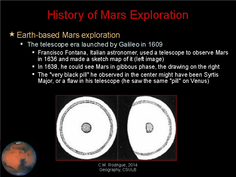
The telescope era was launched by Galileo in 1609 (though others have a good claim on the invention of the telescope). Early telescopists were fascinated by Jupiter and Saturn and there was less exploration of Mars. Francisco Fontana in Italy (one of those claiming to have created a telescope in 1608) turned his telescope onto Mars in 1636 and made a sketch map of what he saw: A bright disk with a line paralleling its limb and a "black pill" in the center. In 1638, he was pleased to report seeing Mars in gibbous phase. The astronomical community had figured out that a planet beyond Earth, visible through reflected light, should show gibbous phases because of the angle between it, the sun illuminating it, and the Earth observer. He drew Mars in gibbous phase, again with the black pill in the center. The identity of the black pill has been argued, on the one hand, to be the dark "Blue Scorpion" of Syrtis Major or, on the other, more likely hand, a defect in his telescope lens (Fontana saw a similar black pill on Venus).

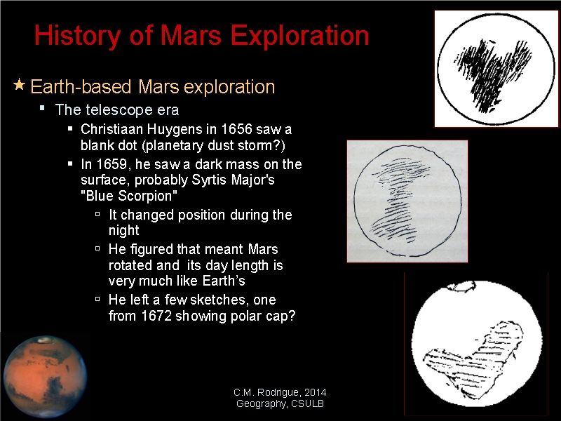
Christiaan Huygens turned a telescope on Mars in 1656 and reported seeing nothing but a blank disk. I wonder if he happened to be looking at Mars during one of its great planetary dust storms that can obscure the surface entirely. In 1659, however, he saw and made a sketch of a dark mass, which was almost certainly the Blue Scorpion of Syrtis Major. The sketch shows a messy triangle, its point directed downward, to the north in the reversed view of telescopy. Huygens reported seeing this dark mass move over the course of the night and inferred that the planet was rotating and its day length was close to that of the earth. He left another sketch map in 1672, which shows, not only the familiar dark (Syrtis) mass but an ellipse outlined at the top of the sketch, possibly the South Polar ice cap.

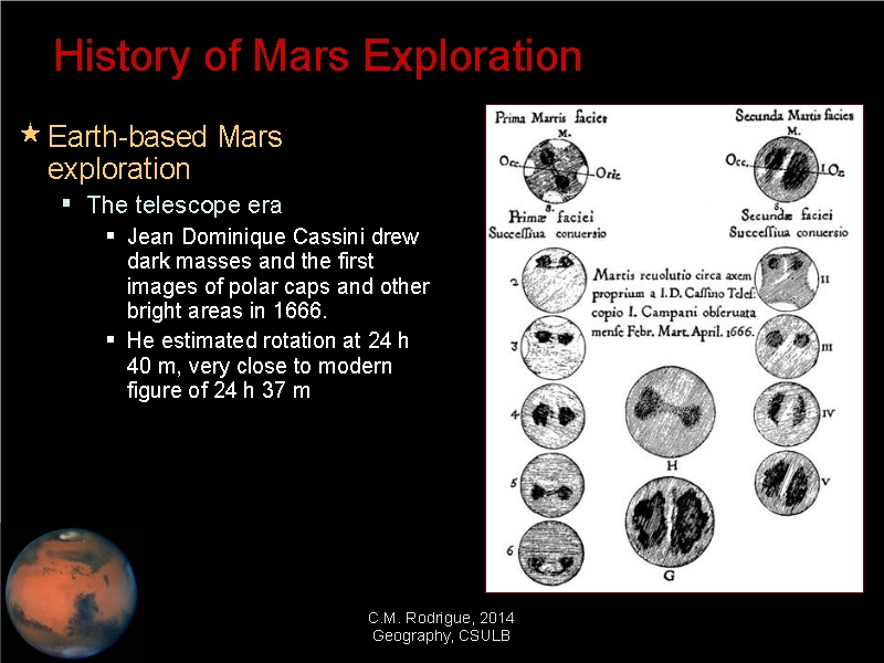
Jean Dominique Cassini left many sketches of his observations of Mars in 1666. These sketches show changing dark masses, sometimes linked together with a dark line or separated by a light line. They also often show as many as four bright areas, perhaps the polar ice caps and possibly other light albedo spots, such as Hellas Planitia. He noted that Mars rotated around its own axis, estimating its daylength at 24 hours and 40 minutes, very close to the modern figure of 24 hours and 37 minutes.

William Herschel built very large reflecting telescopes that were much simplified in design from the Newtonian reflecting telescopes. In 1783, he was able to observe Mars with such detail that he could estimate Mars' axial tilt from the rotation of light and dark areas on the surface (~30°, vs the modern figure of 25°). Noticing the consistent presence of light spots at either end of the axis of rotation and their growth and shrinkage, he explicitly surmised they might be polar ice caps.

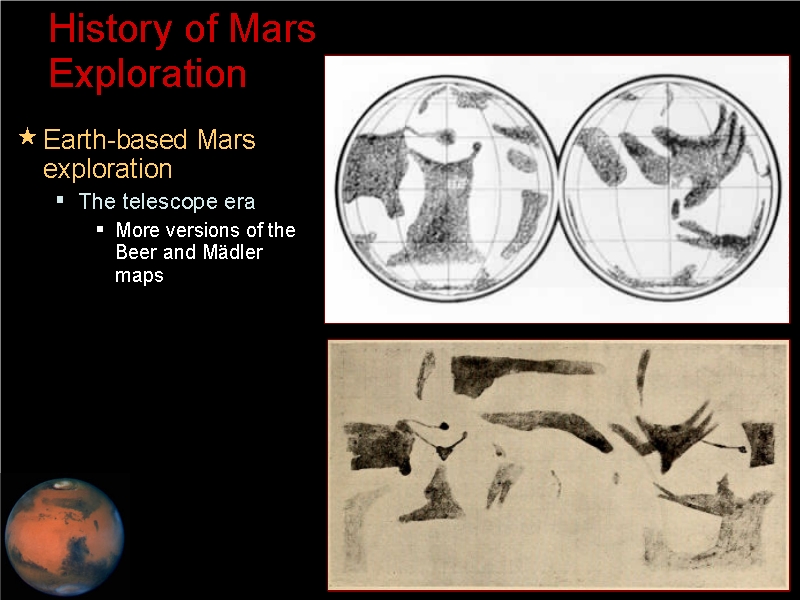
In 1831, Wilhelm Beer and Johann Mädler collaborated to map regularly observed features on Mars, figuring they were probably fixed geological features. They transferred these features to a geographic grid they fashioned for the planet, with a prime meridian in the Meridiani Planum area (hence the name for this feature). The contemporary areographic grid is based on Beer's and Mädler's work, the prime meridian passing through the middle of a small crater, Airy-0, inside Airy Crater. Airy-0 was first spotted in Mariner 6 and 7 images and agreed upon in 1969 as the embodiment of Beer's and Mädler's prime meridian for Mars.

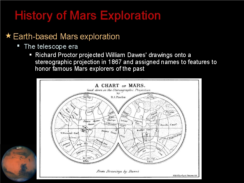
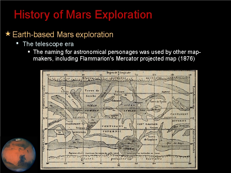
By 1867, so many details had been seen so regularly that Richard Proctor decided to assign names to them. He transferred astronomical drawings by William Dawes onto a stereographic projection and named features to honor famous Mars explorers of the past, such as, well, Dawes Continent and Dawes Ocean, Mädler Continent, Beer Sea, Herschel Continent, and Keppler Land. This idea was appealing to other cartographers, such as Camille Flammarion, who added more details in the spirit of Proctor, such as Huygens Land, Fontana Land, Cassini Land, and, er, Flammarion Sea.

This tradition was superseded by Giovanni Schiaparelli, an Italian astronomer who created several Mercator maps based on observations of the spectacular 1877 opposition. A Mars opposition occurs when Mars and the Earth are on the same side of the sun, in a direct line with one another. In this particular one, both planets were at the perihelion side of their orbits, which brought them within 56 million kilometers of one another. Schiaparelli did a large number of drawings and, when he transferred the markings to the Mercator grid, he assigned names for mythical and historical places on Earth, such as Elysium, Utopia, Arcadia, Hesperia, Arabia, Thaumasia, and Tharsis. He called the thinner dark streaks seen on Mars by then canali, which can be translated as "channels" or ... "canals." Guess which translation stuck? And we were off and running with the first great martian craze: canals on Mars, which could only imply canal-builders. Schiaparelli bequeathed not only the first craze through a gain in translation, but his idea for toponymy stuck. We use a version of his names for various albedo features to the present. When names for features are proposed to the International Astronomical Union, they are checked for consistency with the system based on Sciaparelli.

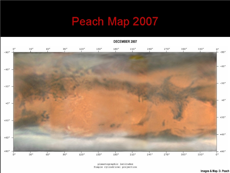
Before I show a couple of the Schiaparelli maps, I'd like to show an impression of what he and others may have been seeing with the well-developed telescopes of the time. There remains an amateur astonomer tradition of observing planets, stars, and other celestial objects and recording one's observations photographically or graphically. One person who does a lot of this and transfers his images to the areographic grid is Damian Peach. Here is one of his maps from 2007, showing south on the top and north to the bottom, as was normal for 19th century Mars cartographers.

Here is the 1877 Sciaparelli map, done fresh after the great opposition. We see the dark areas of the 2007 map and the many bright areas. These are, however, bounded by dark areas and streaks in between them. The modern names are recognizable, such as Hellas, Elysium, Chryse, Thaumasia, and Tharis. Schiaparelli's 1884 map shows most of the streaks as thinner and fainter than in 1877 and also more linear.

Schiaparelli's maps just enchanted Percival Lowell, as did Flammarion's book, La planète Mars et ses conditions d'habitabilité (1892). Lowell was a wealthy Bostonian, who'd spent a lot of his youth travelling, kind of a natural geographer. He came across Schiaparelli's maps and was struck by the concept of "canali." He secured a site in the American Southwest near Flagstaff, Arizona, where the air was stable, to build a major astronomical observatory and equip it with the best instruments money could buy. He spent a lot of his time there observing Mars and making detailed drawings of his observations. He drew great swathes of shaded areas and then lots of long, nearly straight, thin lines criss-crossing Mars in an elaborate spider's web of lineations, with nodes darkened in at many but not all their crossings. He became convinced that the lineations he, Sciaparelli, and many others reported were, in fact, constant features of the martian surface consistent with a canals interpretation, they showed seasonal changes in width and color (perhaps riparian vegetation), and they seemed to go from dark areas near the poles (seas?) to the drier seeming bright albedo areas along the equator.

At the time he was writing, the scientific community had become increasingly aware of profound environmental changes in Earth's past, such as ice ages and desertification. Archæology was framing the collapse of some ancient civilizations to great droughts and the propinquity theory (concentration of plants, animals, and people on oases in a desiccating Middle East) for the establishment of farming and pastoralism. Intelligent life on other planets was a topic of serious conversation. So, Lowell thought that his observations of lineations looked like the kinds of heroic engineering that an intelligent species might try in the face of a desiccating planet seemingly so like our own ancient Middle East. So, at first (1885), he was within the norms of discourse in the scientific community of his time. Indeed, he contributed, not only to advanced telescopic observation and recording of Mars but to the early application of spectroscopy to Mars.

The canals hypothesis began to run into a wall of criticism. Alfred Russell Wallace pointed out that spectroscopy indicated Mars was stunningly cold, about -35° F, which would rule out canals of liquid water. Other scientists reported having trouble seeing canals or any kind of lineations. As peer criticism mounted, Lowell began to shy away from peer review and went directly to the public to press his case in books with such titles as Mars and Its Canals (1906) and Mars, the Abode of Life (1908). He began to drift into pseudoscience, leaving behind an enduring legacy of science fiction and a tradition of popular culture crazes about Mars.

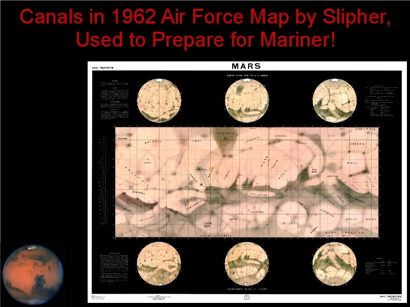
The canals or at least lineations Powell discussed endured in cartography as well. In 1962, Earl C. Slipher prepared a map of Mars at the behest of the U.S. Air Force, which was used to plan the Mariner flyby missions of 1965 and 1969. This beautiful map is replete with faint, narrow, straight shadows.

Contemporary Orbiter-Based Maps of Mars

There now exist several global-scale maps of Mars, based on imagery from Mars orbiters since Mariner 9 (1971-1972). A great contribution came from the Viking mission's two orbiters, which carried the Visual Imaging System, which consisted of a pair of television cameras. These produced overlapping images 40 km by 44 km in surface coverage from 1,500 km up. They yielded nearly 50,000 images with pixel resolution between 150 and 300 m (and some areas were imaged at 8 m resolution). The results included a digital terrain model and the Mars Digital Image Model.

Mars Global Surveyor was the first successful mission to Mars after Viking, operating from 1997 to 2006. Among its instrumentation were three standouts for the cartography of Mars:

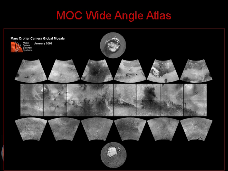
• Mars Orbiter Camera (MOC), which had one narrow-angle high-resolution camera (1.5-12 m resolution) and two wide-angle lower-resolution (230 m to 7.5 km) regional context cameras, one blue and one red. A global map of Mars was produced as an interactive portal to access detailed images of Mars, projected onto a Mercator projection or, as here, divided into the standard thirty "quadrangles" for Mars, the sixteen equatorial quadrangles shown in Mercator, the twelve mid-latitude quadrangles shown on a Lambert-Conformal Conic projection, and the two poles on a Polar Stereographic projection. By clicking on any of the quadrangles shown here (or here for the Mercator version), you are taken to a MOC mosaic of that particular region.

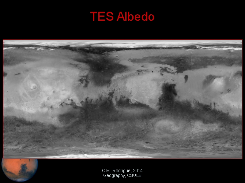
• Thermal Emissions Spectrometer (TES) infrared albedo map. The absorption of infrared radiation by the basalts that also absorb much of the visible light spectrum and the strong reflectance of dust that also appears bright in visible light makes for a gorgeously detailed map of albedo differences.

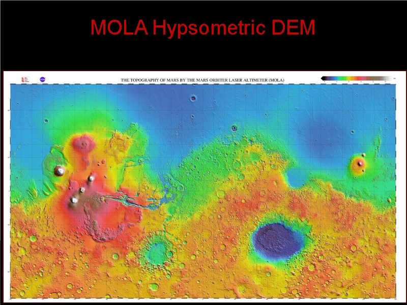
• Mars Orbiter Laser Altimeter (MOLA), which captured laser pulses emitted from the MOLA instrument as they reflected back up to MGS. The delay in time from emission to captured reflection was multiplied by the speed of light to gauge the distance from the spacecraft to the surface. The result was an extremely detailed digital elevation model of Mars. During its lifetime (until June 2001), MOLA took 671,121,600 individual laser pulse measurements, yielding the most detailed elevation model for ANY planet in the solar system, including our own! MOLA was the basis of a number of maps.
  • The most common representation of the MOLA digital elevation map shows the extreme elevational contrast of Mars (from 8.2 km below martian "sea level," or the gravitationally equipotential surface, in Hellas Planitia to 21.2 km above the equipotential datum on top of Olympus Mons) as a hypsometrically tinted map. The color ramp ranges from black through purple, blue, green, yellow, orange, red, brown, and beige to white. Dr. Tyner, on seeing this, commented that it's a "propaganda map" or, more kindly, an example of "persuasive cartography." No doubt innocently applied, this color ramp feeds into the discussion of whether Mars ever had oceans. Looking at this color ramp, the Northern Lowlands and Hellas Planitia fairly scream oceans!
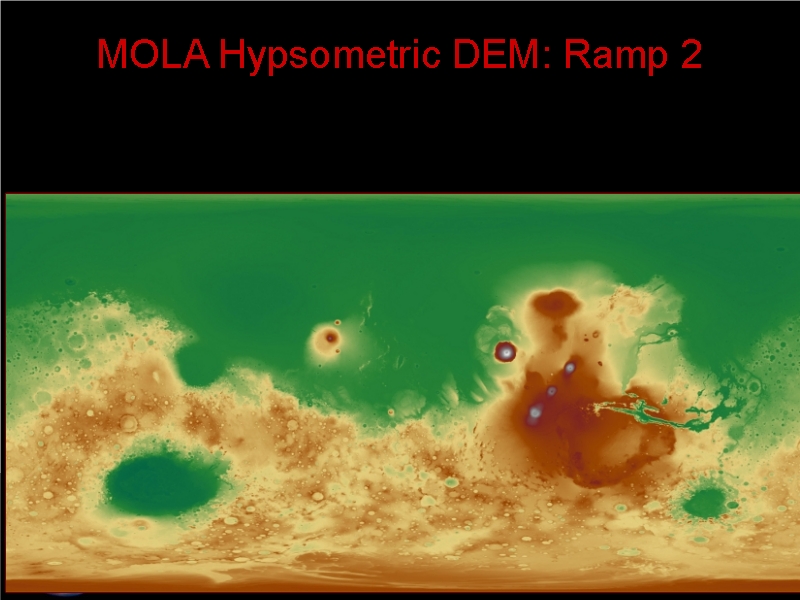
  • Another ramp was used in a rendering of the MOLA DEM by Kevin M. Gill on his Apoapsys blog. It shows the lowlands in green and the uplands in brown, much like the hypsometrically tinted elevation maps of Earth. This creates an oddly "familiar" Mars.
  • Daniel Macháček has produced another rendering of the MOLA DEM in hypometric tints, this time ranging from aqua to brown, muted like the Gill rendering but still visually persuasive of oceans on Mars.
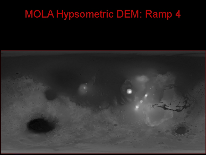
  • Gill did another rendering of the MOLA model, this time in greyscale, ranging from black to white. This is a lovely rendering, echoing the appearance of the greyscale in which the MGS MOC and Viking VIS captured panchromatic images of Mars or images confined to particular bands and yet clearly indicating the elevational contrasts of Mars.
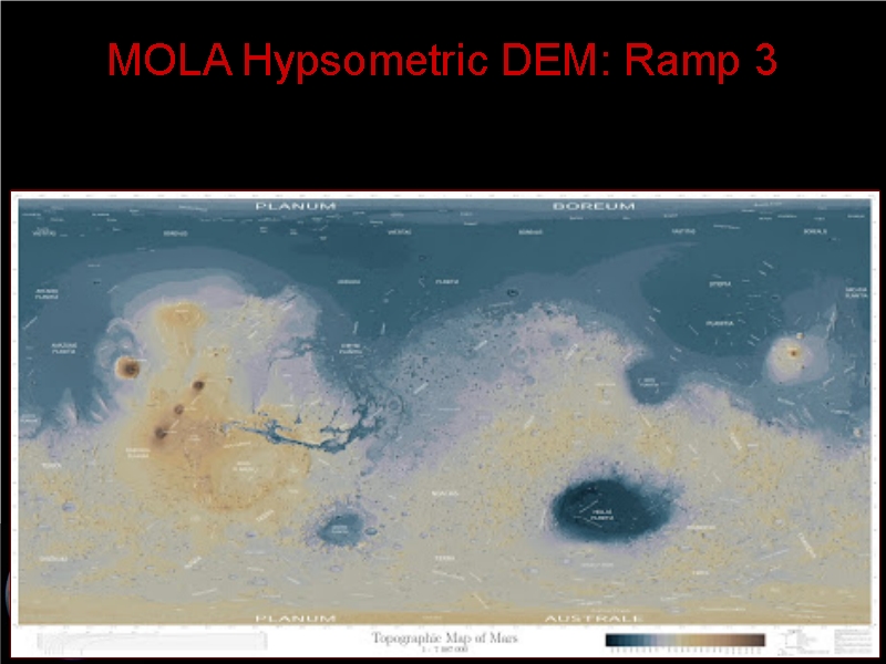
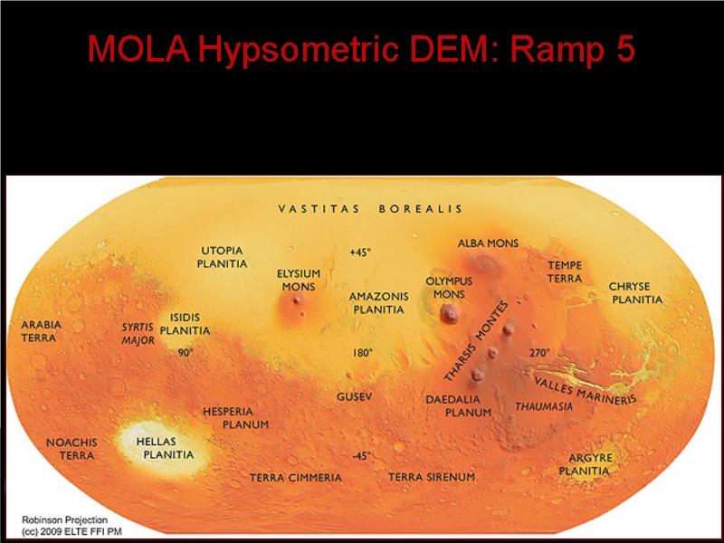
  • Henrik Hargitai is a prolific planetary cartographer in Hungary, and he has produced exquisite maps of Mars based on the MOLA DEM and shaded along a color ramp running from light yellow through an ochre brown. The map conveys the topographic information provided by MOLA but in tints reminiscent of the colors on the Mars surface.
  • The MOLA DEM has also been represented, not as a contour map hypsometrically tinted, but as a shaded relief map, again a stunning visual representation of the planet. The image is less likely to evoke thoughts of martian oceans.
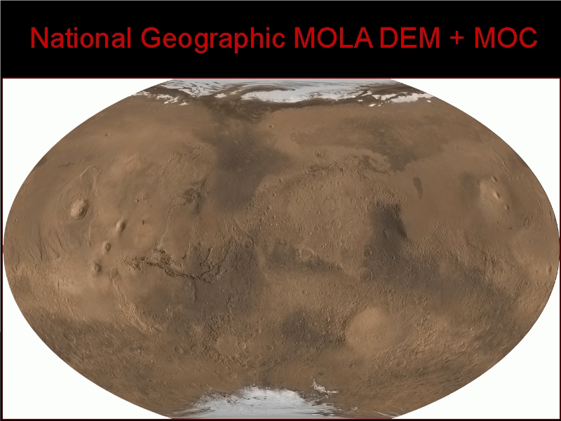
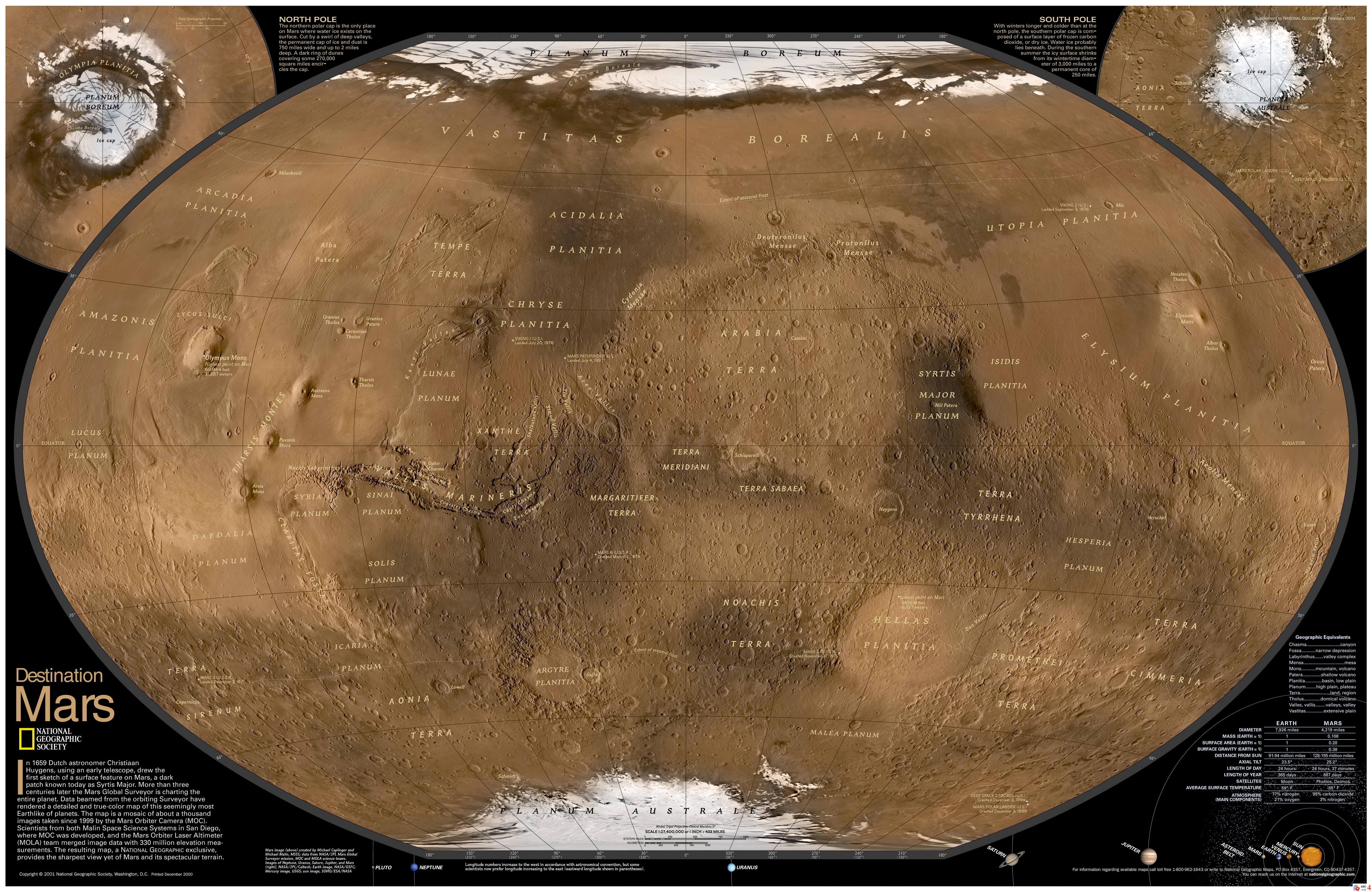
  • National Geographic produced a stunning map in 2001, which combined the MOLA DEM with a true-color MGS MOC image mosaic. Here is a link to a version of the National Geographic map with place names.
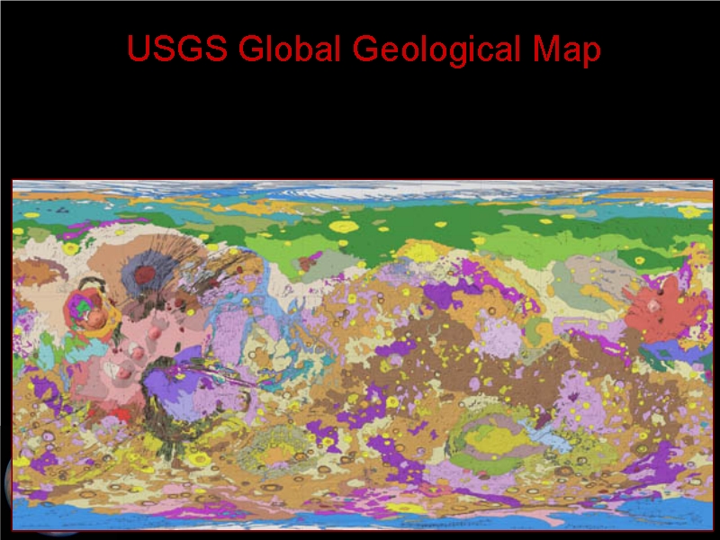
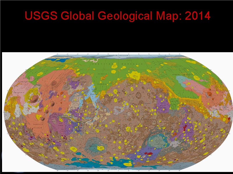
• The U.S. Geological Survey has done geological maps of moons and planets on behalf of NASA since 1963. Here are geological maps of Mars, the first based on analysis of Viking Orbiter images and the most recent an update including data from NASA's Mars Global Surveyor (1997- 2006), NASA's Mars Odyssey (2001-), ESA's Mars Express Orbiter (2003-), and Mars Reconnaissance Orbiter (2006-).
  • Viking-based geological map of Mars (1986)
  • Geological Map of Mars (2014).

The Orders of Relief Scheme

One of my main student learning objectives in the Geography of Mars class is construction of a vivid mental map of Mars. To develop a sense of Mars as a place, I decided to present its regions in a (mostly) nested hierarchical scheme. This is modelled roughly on the Nevin Fenneman "Physiographic subdivision of the United States" model presented in the Annals of the Association of American Geographers back in 1916. This idea of nesting progressively finer areal units in coarser scaled ones has taken on a life of its own in many introductory geography courses to the present day. On Earth, the orders of relief scheme might represent the first order as the division between continents and oceans. The second might be great physiographic divisions, such as the Atlantic Plain or the Pacific Mountain System. The third would be geomorphic provinces, such as the Pacific Border Province, nested in the Pacific Mountain System. The fourth might be Fenneman's sections, such as the California Coastal Ranges, nested in the Pacific Mountain System.

For Mars, the first order would include the great crustal dichotomy between the smooth Northern Lowlands and the intensely cratered Southern Highlands. Another would be the great Tharsis volcanic rise, which occupies about a quarter of Mars' surface area. The second order is made up of the large, visually distinctive features that can be used as the framework for a mental map by allowing easy positioning of other features by reference to one or another of these features (e.g., "Promethei Terra lies to the southeast of Hellas Planitia"). Because of their function in framing the rest of martian geography, they often do not nest tidily within the first order features. The third order would be large regions, some of them bigger than the second order features but less obviously distinct. I used the third order to introduce the martian geological periods and how they are determined by relative density and sizing of craters. These nest within the first order features. The fourth order would be smaller features nested within third order features, comprising landscape scale features. Fifth order features would be small features at the scale of the landers' and rovers' activities or the fine-scale imagery from orbiters. These would nest within the fourth order features.

Hoping to improve my presentation of this scheme in the Spring 2015 offering of the Geography of Mars class, I've been working on maps delineating these features' boundaries, using broad, fuzzy lines to express the statistical and geological uncertainty in defining their boundaries. To do this, I used the MOLA white-brown-red ... blue-black hypsometrically tinted MOLA map as the base, importing it into an open-source graphics program called GIMP (GNU Image Manipulation Program; I used GIMP 2.6, but 2.8 is now available). GIMP allows line and polygon delineation as "paths," which can be "stroked" with various brushes, and the stroked lines saved as separate layers above the background image. These can be hidden or shown as wanted. Various layers can be made visible, togehter with the background image, and the visible layers can be output as JPEG or PNG image files. I eventually used more than 30 paths to define each of the regions at the first, second, and third orders of relief and displayed them as over 30 stroked line layers. Each path and each layer is named for the feature in question. If you would like to open this image, first download GIMP, then the image file, and then open the image file in GIMP. The default mode should show the Layers, Channels, and Paths toolbox beside the image, and you can use the layers button (looks like a stack of papers) to open and close various layers to see the scheme. The image file is at https://home.csulb.edu/~rodrigue/mars/regions/mercatorMOLApaths.xcf.

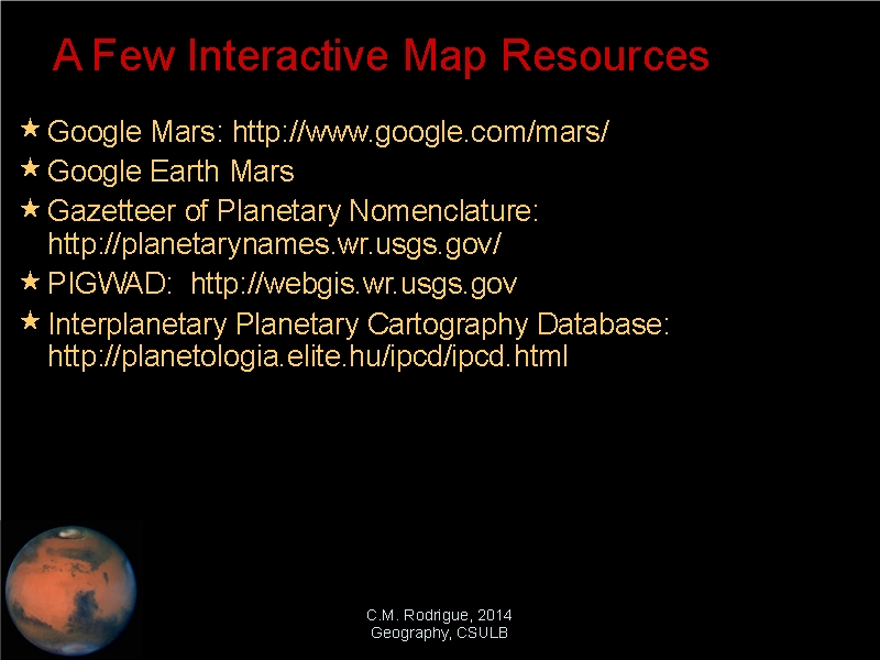
A Few Online Interactive Map Resources

The Internet has enabled interactive mapping of Mars. This allows the reader to learn the locations of place names on Mars and the topography and geology of Mars at adjustable scales. Here are a few to get you started on your own explorations of Mars:

• Google Mars
• Google Earth Mars
• Gazetteer of Planetary Nomenclature (Mars)
• PIGWAD
• International Planetary Cartography Database