GEOG 442 biodiversity lab: Dr. Rodrigue

GEOG 442

Biogeography

Analysis of Biodiversity Patterns

In this lab, you'll examine species richness counts for different organisms in different locations on the North American continent to see if you can pick out environmental gradients that co-vary with the species richness gradients. Some of these run more or less north-south and others run east-west. It might help if you consulted an atlas while doing these analyses, as regional context gives clues. Your biogeography text and notes and any introductory physical geography or environmental science text would be helpful resources, too.
Note: Directions are for LibreOffice Calc. You can do it in Excel if you prefer, but you have to figure out equivalent processes in Excel). LibreOffice Calc is virtually identical to OpenOffice Calc, which are forks from the same open-source software project, but LibreOffice Calc can fit a higher-order polynomial trendline to your scatterplot, which is especially useful for the mammalian quadruped density graph. You'd ask it to fit a trendline and then select the polynomial type and then fiddle with the order of the polynomial (try 4, 5, or 6 to find the best one).
If you'd like to do this at home instead of one of our computer labs, you need to download LibreOffice. It's free! You can do that at https://www.libreoffice.org. You'll get a full featured office suite, with spreadsheet, word processor, viewgraphs program, database, graphics program, and even an equation editor. Did I mention that it's free (and generally easier to use than the commercial one)?
Lab deliverables include:

Your answers to the questions in the lab (it's okay to print it out and fill it out by hand but you'll save on dead tree by firing up your word processor (LibreOffice has a nice one called Writer) and composing your answers in a separate document, into which you could insert your scatterplots)
Your four scatterplots (you can do a page preview in Calc and then arrange their size and location to put them on two pages and then just print those two pages from Calc

Getting Your Data
To get the data on which this lab is based, click here. It should just open up in LibreOffice if you are in our lab. If not or if you are doing this at home after downloading LibreOffice, you may be asked instead what to do with the file. Select Save File As and then specify where you'd like to keep it. If you're doing this at home, stash it anyplace you normally keep data. If you're in our labs, please save it to your own flash drive, because the student files on the "thaw drive" system are purged frequently. Alternatively, you can risk saving it on the Thaw Space (T:\) and then try to remember to e-mail it to yourself before leaving the lab.

Mammal Quadruped Diversity in Central and North America

Now you have your data, what do you do with them? First, take a look at Columns A and B, the ones highlighted in light blue. Column A shows the latitude of 22,500 square mile quadrats throughout Central and North America. Column B shows the number of mammalian quadrupeds that showed up in species counts within each of those quadrats. To see the pattern in the numbers, first highlight cells A4 through B51.
Now, select the chart button from the Calc toolbar on top on the right side (it looks like a little bitty pie chart done in garish colors). This activates the chart wizard dialogue box.
Under Choose a chart type, pick XY (Scatter) and then select the box that shows a bunch of dots on an X-Y graph without any lines connecting them (leftmost choice). Then, select Next > from the buttons on the bottom of the chart wizard.
Accept Data Range (from highlighting A4:B51 earlier) and indicate that the series is in columns. Then, hit Next > again. You don't need to Customize data ranges, so hit Next again. Under Titles, come up with a name for your chart and enter it in the Title box. Under X axis, put latitude. Under Y axis, put in # of spp/quadrat. If you're feeling fancy, you can play around with Gridlines and Legend, but you don't really need to. In fact, you can disable the Legend function, as it's kind of pointless here.
Click Finish and poof! the graph pops up in your spreadsheet somewhere, probably someplace inconvenient.
The graph is editable if you see a grey border with black dots on the edges. If it isn't editable, just double-click on it until you see the grey borders.
You can click outside the graph and then click the graph once: That creates green dots on the border, which allows you to move it without editing it or copy it.
You can move it wherever you like in edit mode by putting the cursor on the grey border, holding down the left mouse button, and dragging the whole thing where you want to put it.
You can move it in non-edit mode (green boxes) by putting the cursor anywhere in the graph and dragging. You can even delete it in non-edit mode and then go to Sheet 2 and paste it there.
You can then fiddle with the shape of it in either mode, too. By clicking on one of the border boxes, you can stretch or compress the whole graph so that it takes on a pleasing shape.
To see it readily, you might want to exit edit mode, click the graph once (green buttons), hit Format, then choose Graphic, and then Line. In the Line tab, click the Line Properties Style box and pick Continuous, the Color you'd like and a width (probably 0.02" is fine). That will create a "neat line" around it.
You can get pretty fancy. Double-click on the graph in one of the blank areas near the corner to put it in edit mode. That will activate it for customizing (grey borders and black dots framing the graph). Then, right-click in that corner and ask to Format Chart Area, picking the Area tab and picking a color you like. That will paint the whole thing. You can right-click inside the chart wall and choose Format All and color that area white or some other contrasting color. You can click on one of the dots in your scatterplot and, again, you can fiddle with color, shape of symbol, size of symbol, etc., in the Format Data Series option.
That done and the graph looking mighty purdy, you can touch one of the dots again, right-click, and then pick Insert Trend Line. Under the Type tab, you can experiment in here to your heart's content. The Linear option doesn't do a good job on the wavy pattern of dots you get. To capture that undulating pattern, pick Polynomial, and then experiment with different orders to fit the curve pretty close to the trends in the dots.
When you're happy with it, have a look at the pattern you've created.
In simple English, what is the relationship between latitude and species richness? Is it direct (increasing with latitude) or inverse (decreasing with latitude)?
_____________________________________________________________________________ _____________________________________________________________________________ _____________________________________________________________________________
Now, the hard part. Why do you think this relationship exists? What is it about latitude that might affect species richness? You may want to rummage around in your notes or in Chapter 2 of Cox, Moore, and Ladle for some ideas. Use the bends in the trendline and figure out where (location on map) the species richness peaks (latitude ranges).
What is found in the global air circulation pattern at the latitude of the first drop, which could limit biodiversity? Compare this map of the world pressure and wind bands with the latitude of that first drop in biodiversity: http://geologycafe.com/images/world_wind_zones.jpg. What kind of climates are associated with that drop in diversity?
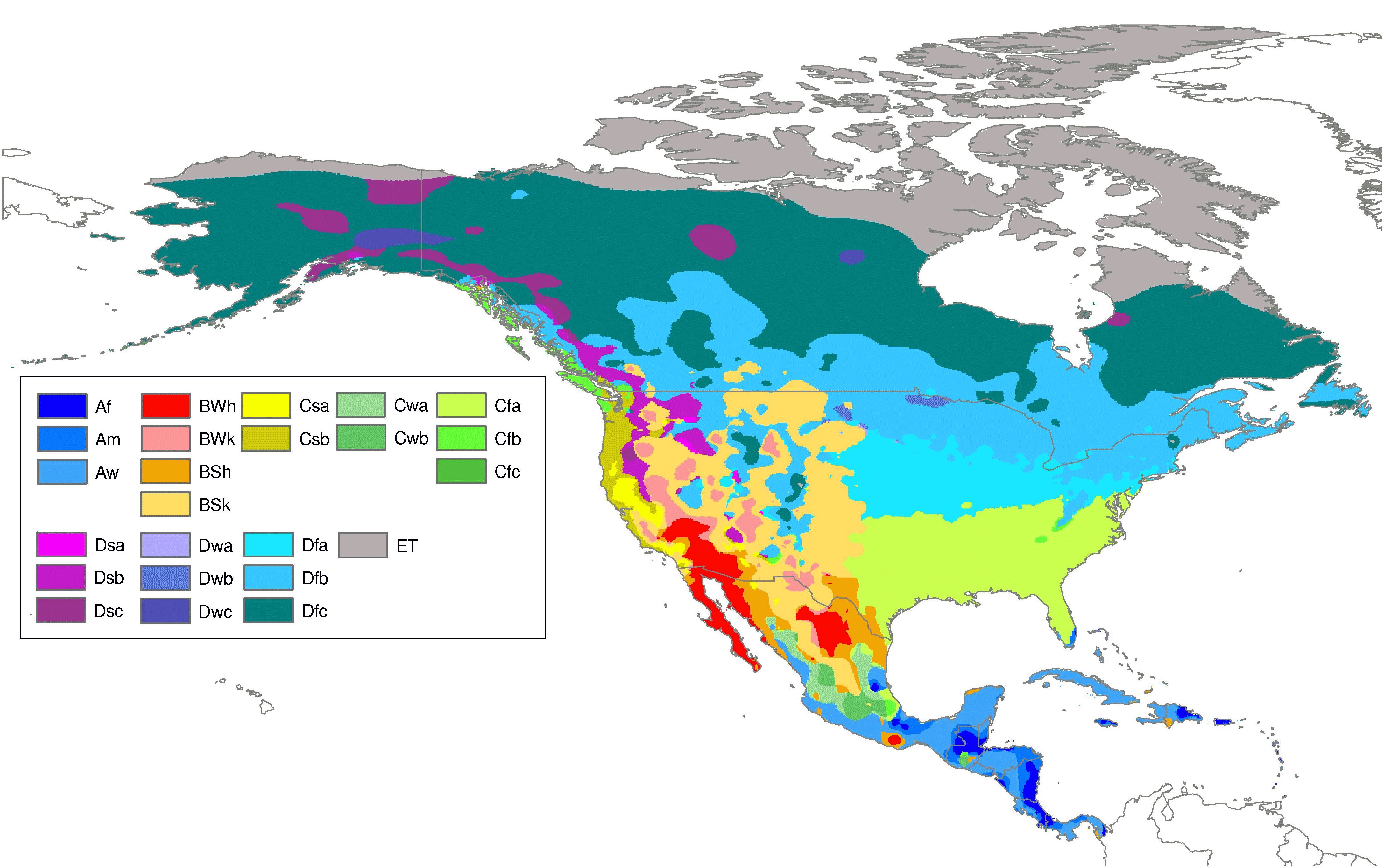
Notice how and where that pattern eases off and plateaus. What kinds of climates are found in those latitudes (first letter code of the Köppen- Geiger classification)? Some maps might help: Here is a global map of Köppen-Geiger climate types: http://koeppen-geiger.vu- wien.ac.at/pics/kottek_et_al_2006.gif. And here is one just of North America: http://people.eng.unimelb.edu.au/mpeel/Koppen/North_America.jpg. Here is a succinct general description of the codes: https://www.mindat.org/climate.php.
Again, the plateau/sub-peak ends and biodiversity slides downward again. What is going on in the latitudes of that second drop in diversity? Lab 1 might be helpful here.
But, again, the biodiversity plateaus out yet again before making its final drop. Why would biodiversity form this third plateau/sub-peak at such high latitudes (Lab 1 ...)?
_____________________________________________________________________________ _____________________________________________________________________________ _____________________________________________________________________________ _____________________________________________________________________________ _____________________________________________________________________________ _____________________________________________________________________________
Now, look at the deviations of dots from your polynomial trend line a little more closely. In which latitudes do you find the dots are the closest to the trendline describing them? There is one area, however, where the dots diverge quite a bit above and below the trendline. What is that latitudinal band (focus on perhaps the 2 most divergent outliers)? So, you have a site more biodiverse than it "should" be and another way less diverse. Which side of the United States do you suppose the superdiverse site is on and which side is the underachiever on? What do you know about the climates on the east and west ends of the US in those latitudes (see map and climate code descriptions above)? Think about the seasonality of their precipitation. Speculate on the degree of departure from the polynomial regression line and what's going on in that 30° - 40° zone.
_____________________________________________________________________________ _____________________________________________________________________________ _____________________________________________________________________________ _____________________________________________________________________________ _____________________________________________________________________________ _____________________________________________________________________________

Tree Richness Gradients along Transects in North America

In columns F, G, H, and I of your spreadsheet, you have latitude and longitude and species richness data for ten locations along each of three transects, or sampling lines. Each location is roughly in the center of a large quadrat (70,000 square kilometers). The number of species of trees that were counted within those quadrats is given. You'll notice that for each quadrat, either latitude or longitude (Column G) is more or less the same: The top set of ten comes from a transect running from the West Coast at roughly 37° N to the East Coast at roughly 33° N. The two transects below it run due north/south, one at 118° W and the other at 80° W.
First, let's deal with the W/E transect. Highlight cells H4:I15. Again, you'll create an X-Y graph by activating the Chart Wizard. Again, pick XY (Scatter) and then select the Scatter with data points connected by lines option (second choice) and hit Next. Make sure that Data series in column and First column as label are checked but First row as label is not. Again, hit Next and Next.
In Titles, name your chart in Chart title. Value (X) axis should read longitude, while Value (Y) axis should read # spp/quadrat. hit Finish. Again, move your chart where you want and morph its shape to make it somewhat æsthetic. Unleash your inner artist if you like.
In clear English, how might you describe the relationship between longitude and species richness along this west to east transect across the United States?
_____________________________________________________________________________ _____________________________________________________________________________ _____________________________________________________________________________
What is going on along that transect that might affect richness? Again, the Köppen-Geiger map might be helpful.
_____________________________________________________________________________ _____________________________________________________________________________ _____________________________________________________________________________ _____________________________________________________________________________ _____________________________________________________________________________ _____________________________________________________________________________
Now, do the same for the second transect, which runs from Southern California to Canada's Northwest Territories along the 118° meridian. This time, your data range runs from H18 to I27, and you'll use latitude as the label for the X (horizontal) axis.
Briefly, how might you describe the relationship between latitude and species richness along this south to north transect across the United States along this western meridian?
_____________________________________________________________________________ _____________________________________________________________________________ _____________________________________________________________________________
Once more, with vigor, do a graph for the third transect. This one runs from Florida to Baffin Island along the 80° meridian, and your data range from H30 to I39. The X axis will be labeled latitude.
Again with terseness, how might you describe the relationship between latitude and species richness along this south to north transect across the United States along this eastern meridian?
_____________________________________________________________________________ _____________________________________________________________________________ _____________________________________________________________________________
Now, the fun part: Compare and contrast the patterns you see along these two north/south transects. It might help if you format each X axis so that it runs from 25°N to 75°N, so you can compare them, latitude by latitude. Also format the Y axis on the West Coast transect to run from 0 to 180 (not 90), so it, too, matches the East Coast transect chart.
How do the two patterns resemble one another? What might be driving that similarity?
_____________________________________________________________________________ _____________________________________________________________________________ _____________________________________________________________________________
In which ways do they differ? Look especially at the shape of the drop off in species (where they're concave and where they're convex and the latitudes at which these deviations from a straight line relationship take place).
_____________________________________________________________________________ _____________________________________________________________________________ _____________________________________________________________________________
What is going on to explain the differences in the two latitude/richness curves? You may need to dust off your introductory physical geography textbook (what? you sold it?! how could you DO that?!!!) for clues somewhere in the climate section.
_____________________________________________________________________________ _____________________________________________________________________________ _____________________________________________________________________________ _____________________________________________________________________________ _____________________________________________________________________________ _____________________________________________________________________________ _____________________________________________________________________________ _____________________________________________________________________________

first placed on the web: 11/03/03
last revised: 02/18/19
© Dr. Christine M. Rodrigue