The Geography of Mars

Using the Hartmann-Neukum Isochron Histogram to Estimate Surface Ages

This lab has the following objectives:

• to familiarize you with crater-counting as a way of constraining the ages of surfaces on Mars
• to do so, using the size-frequency isochron system developed as a compromise between the Hartmann (three different regressions) and Neukum (higher-order polynomials) approaches
• to have you plot crater frequencies by size bin onto the Hartmann-Neukum graph
• to have you estimate the ages of different martian surfaces
• to introduce you to a great crater database (and a few other useful resources en route)!
• to prepare you for a guest lecture and demonstration by our own John Adrian, who has become familiar with CraterStats, the latest development in crater-counting, which lets you use a variety of methods to estimate surface ages on Mars that are not confined to the somewhat artificial concept of histogramming craters by arbitrary bins sizes.

Background

As with many hazards, there is an inverse relationship between the size of an event and the frequency with which events of that size or larger recur (magnitude-frequency relationship). Crater diameter and frequency relationships very roughly follow an inverse power law relationship:

N = aD^-b or, alternatively, log₁₀N = log₁₀a + b(log₁₀D)

Where:

• N = Number of craters ( in or above a given size bin)
• D = Diameter of a crater's rim
• a = an empirical constant that you calculate to represent the Y intercept or where on the Y axis the line describing the association crosses (the higher the intercept, the older the surface)
• b = an empirical constant that you calculate to represent the slope of the trendline

As we discussed in class, b varies along the size-frequency relationship. On Mars, it averages roughly -1.8 for craters between about 1 km in diameter and 64 km.

When you plot the crater size and number relationships on Mars, however, you find that the curve does not perfectly follow the line predicted by the power law regression. The actual curve turns down or steepens past ~64 km (b becomes -2.2), reflecting the fact that by ~3.7 Ga (gigayears or billions of years), nearly all the big objects that had accumulated in the solar system and then sent inward by changes in the gas giants' orbits had already smacked into one of the inner planets and were no longer "available" to provide giant cratering "services."

The curve also steepens substantially below ~1 km (b becomes -3.82). This might reflect some heightened availability of smaller objects (e.g., breakup of larger bolides in Mars' atmosphere, resulting in multiple smaller primary craters), but it might reflect secondary cratering, or craters caused by debris shot upward and outward during a primary impact. These would necessarily have a smaller size distribution than primary impactors, accounting for at least some of the turn up below ~ 1 km.

Now that much finer spatial resolution imagery is available from MOC, CTX, HiRISE, HRSC, THEMIS, and others, another change in the slope of that size-frequency curve has become apparent below ~63 m, a slight flattening of the curve. This probably reflects the gradual erasure of smaller craters by various geomorphic processes on Mars: While not as geologically active as Earth, Mars is vastly more active than our Moon.

There have been all kinds of approaches to cooking the math to make it fit Mars plots, including recalculating b for different segments of the curve (e.g., Hartmann) or fitting a higher order polynomial curve to account for all the bends (e.g., Neukum). Another plot complication involved coming up with absolute ages for the relative differences in crater size distributions from one place to another on Mars. This entailed using the lunar rocks brought back by the Apollo Moon landings, which could be radiometrically dated and their source regions specified on the Moon's variously banged up surfaces. Now, the size-frequency distribution would have to be different for Mars than for the Moon, because:

• Mars is much larger than the moon, so it has greater gravitation, which would accelerate the velocities of incoming bolides.
• Mars has an atmosphere, which would also affect the velocities of impact, but by slowing them a bit.
• The atmosphere would also cause more frictional ablation and shattering or detonation of incoming objects, especially smaller ones.
• Mars is also closer to the presumed source of most of these impactors: the asteroid belt between its orbit and Jupiter's. This might provide more impactors than the moon has experienced.

So, the size-frequency distribution was adjusted for these effects and that allowed at least a ball-park estimate of actual absolute ages. The adjustments are described at https://www.psi.edu/epo/isochrons/chron04b.html. The general idea behind the Hartmann-Neukum isochron approach is sketched out at https://psi.edu/epo/isochrons/chron04a.html.

It was quite a little controversy in the 1990s until Hartmann and Neukum decided to create an isochron graph that incorporates both their approaches so that people doing processual analyses on Mars can have a handy, portable scheme for estimating surface ages, simply by reading isolines of equal age, or isochrons. I modified that a bit to show gridlines to make it easier to enter calibrated crater counts on this common-log by square root of 2 chart if you were doing this by hand. Which you're not.

Your data and methods

First, get your data:

• https://www.google.com/mars/. This is a MOLA-based map of Mars to do some basic orienteering (Google Mars). Look around in here to become familiar with potential study sites you can use: very smooth (young), moderately cratered (middle age), and heavily cratered (ancient).

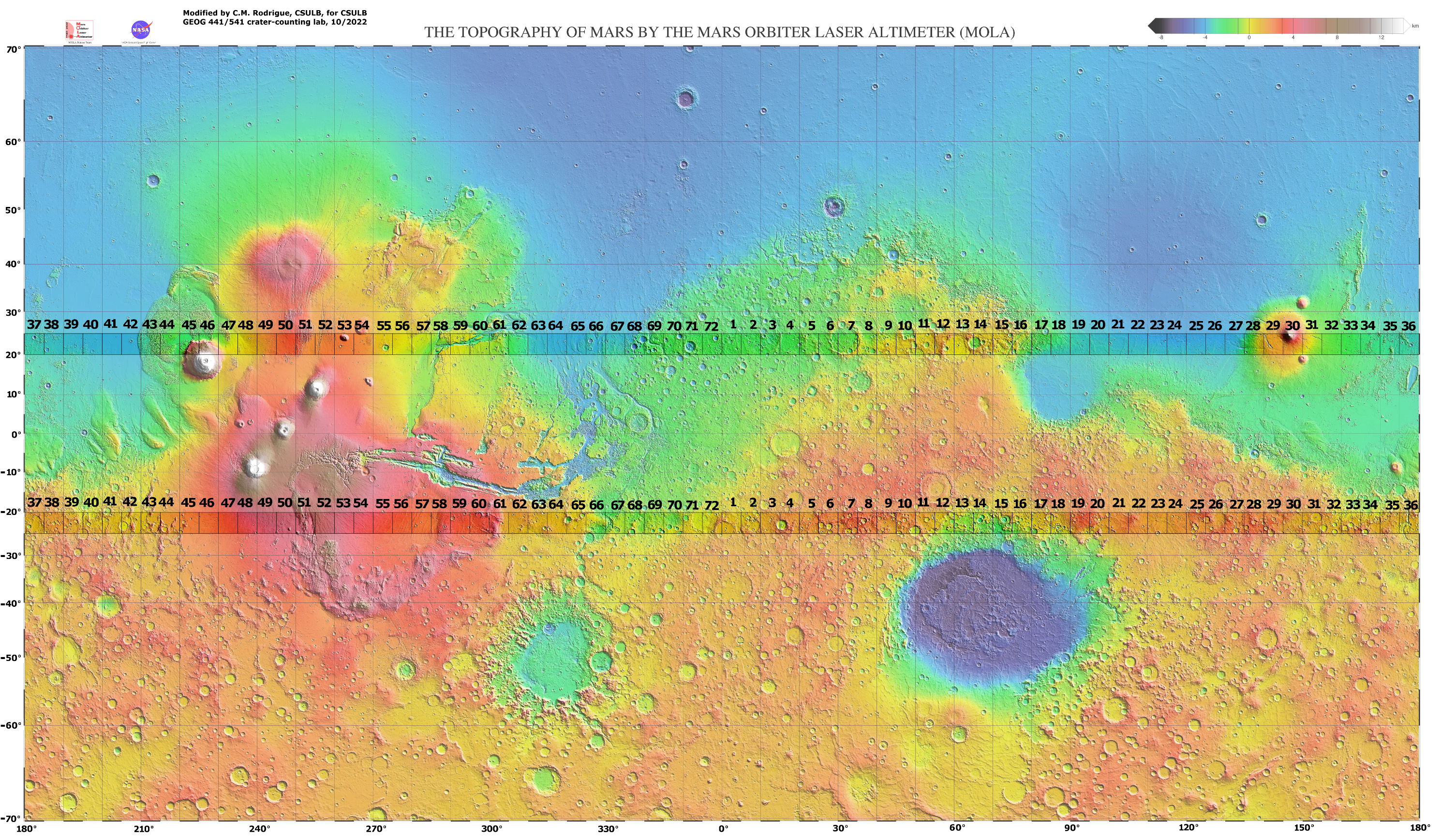
• https://home.csulb.edu/~rodrigue/geog441541/labs/cratercounting/MOLA_mercat_CClab.png. This is a MOLA map I modified to draw your attention to the two 5° latitude bands (20°N to 25° S and 20°S to 25° S). By focussing on just this one latitudinal extent in each hemisphere, I'm reducing the amount of math adjustments you need to do. I've coded each of the 72 longitudinal bands with a number, counting upward east from the "Prime Meridian" in Meridiani Planum: You'll see both latitudinal "stripes" use the same codes. After your general impression from Google Mars, rummage around in this map to pick three squares that embody young, middle, and old ages, based on how crater-hammered they look. Note the longitudinal code and whether your squares are in the northern or southern bands.

• https://home.csulb.edu/~rodrigue/geog441541/labs/cratercounting/CraterCountsLab.ods. This is the database you need for this lab, which simply presents the counts by size bin and by longitude (the study areas are all 5° wide) and in two groups: the Northern Hemisphere band and the Southern Hemisphere band. Look up your three chosen squares: You'll find all the craters in those squares are already binned and counted for you.

• https://home.csulb.edu/~rodrigue/geog441541/labs/cratercounting/Isochron04Auto.ods. Now, fire up my infamous crater counting spreadsheet, in which I tried to automate the Hartmann-Neukum isochron approach to estimating ages. Make sure you're in the Data Entry tab and that the sheet is centered on Column U, the blue-shaded one where you can enter your count data. There are probably numbers there already -- it's okay to override them. Also, make sure the left window shows Column A, which is the boundary for each of the square root of 2 bins that Hartmann and Neukum use, just so you know where to plop your data. Go back to the CraterCountsLab spreadsheet and highlight the crater frequency corresponding to one of your chosen study areas. Copy those counts (Control-C). Now, back in the Isochron spreadsheet, put your cursor on the blue shaded line corresponding to 1.0000 km shown in Column A (the smallest craters Robbins included in his database). When you're sure you're in the right blue cell, hit Control-SHIFT-V to plop your craters in the right place without screwing up the format of the Isochron spreadsheet. A lot of magic happens; don't look at the purdy picture just yet!

We need to get our crater frequencies calibrated to the number of craters per square kilometer that Hartmann-Neukum uses (that goofy concept of how many 64 km diameter craters fit in our 1 square kilometer). After reading what follows, you'll be thrilled that the spreadsheet will do everything if we give it the parameters it needs.

The overview: We need to divide our crater counts by the area of our study area. Our study areas are 5° on a side, but remember that this is on the surface of a sphere: The more poleward longitudinal mileage is smaller than the longitudinal mileage along the equatorward side. So, we're dealing with a trapezoid, not a square (and even that's not quite enough -- I'm not dealing with the actual rounded surface of our study areas, though at this scale the effect is trivial).

The formula for area of a trapezoid is:

A = h/2 * (w₁ + w₂)

Where:

• A = Area
• h = latitudinal "height" (Mars' average circumference, 21,344 km, divided by 360° times 5°)
• w₁ = longitudinal "width" on the equatorward side (cosine of 20° times h)
• w₂ = longitudinal "width" on the smaller, poleward side (cosine of 25° times h)

Let's let Calc handle all this. Scroll down past the gorgeous (but not yet accurate) graph to cell U105. You'll be entering numbers in the blue-shaded cells.

• We need to tell the spreadsheet which hemisphere our study area is in (write in N or S) in Cell V105).
• What's the latitude closest to the equator in your study area? It'll be 20, so enter that in Cell 106.
• What's the maximum latitude of your study area (the parallel closest to the nearest pole) -- that would be 25, so put that in Cell V107.
• Are you using eastings or westings? I designed this lab to use eastings, so put E in Cell V108.
• What's the minimum longitude for your study area? Write that in Cell V109.
• What's the maximum longitude for your study area? Put that in Cell V110.

Calc plugs all these into the equations described above in the white cells below your data entries. It results in the size of your study area (pink cell). That figure is used to calibrate the crater counts for plotting on the isochron chart (the pretty picture you bypassed until now). The numbers will show up in the pink column beside your raw crater counts (Column T). They, then, generate the pattern of orange dots on your automated isochron chart.

Other areas in the spreadsheet calculated the isochrons for that isochron chart, based on Hartmann's and Neukum's 2004 iteration. What you now get in that isochron chart is a representation of your study area's crater distribution in comparison with ideal distributions for various ages of surface (isochrons). Your calibrated crater counts show up as orange dots in the chart and even some sense of the statistical uncertainty related to the sample size in each bin (red bars above and below the orange dots).

Interpreting your isochron charts

Ideally, all your dots would line up like obedient little ducklings in a line paralleling one of those isochrons. In the real world, you'll see your dots wandering away here and there, especially on the right side (you get crazy small-sample effects and high uncertainties among the largest craters).

Something else going on has to do with the lack of homogeneity in your five-degree study areas. These largish study areas typically include multiple surface units of different ages. You might have an old highland terrain full of large craters but there may have been newer resurfacing in some areas, such as when a fresh lava flow covers part of the older terrain, a newer hydrological process eroded one surface and deposited materials on another, a landslide fell in an old canyon, or whatever. You can use this spreadsheet on smaller units (if you remember to adjust everything in Cells V105 forward), but that imports another problem. As your study area shrinks, your cell frequency counts do, too, and that can result in small sample effects and high uncertainties! Danged if you do and danged if you don't! But crater-counting is IT for constraining, at least loosely, surface ages until some day samples of Mars "stuff" can be brought back to Earth and radiometrically dated and all the crater counts recalibrated with actual martian data.

So, to interpret your crater counts, focus only on the left side of the distribution, the larger counts in smaller size bins. It's safest to focus on the range from about 1 km up to maybe 16 km (about the length of that thick, short isochron marking the transition from the Noachian to the Hesperian a bit before 3.5 billion years ago. Focussing just on that, about how old is the bulk of your study area? Compare the nearest isochrons in the vicinity of your small-diameter bin counts to constrain the age range in your study area.

What your graph shows is the famous magnitude-frequency curve seen in many natural (and sociogenic) hazards, such as flooding, earthquakes, volcanic eruptions, industrial toxic release accidents. And this includes the hazard of extraterrestrial bolides hitting Earth, too!

Deliverables

You can keep a record of your study area (and share them with me). There's a tab on the bottom (you may need to move the left window and then widen the scrollbar to see it) called Print Graph. It duplicates your isochron chart and fills in data about your location. The spreadsheet sometimes refuses to print this. What you can do is take a snip or screenshot of it and upload it to BeachBoard. In the comment area on BeachBoard's Dropbox, tell me the general age ranges of each of your study areas (e.g., "between 3.5 and 4.0 Ga") and whether the youngest area shows a younger age (dots lower on the chart) than the oldest area does (dots higher on the chart), based just on the 1 km to 10 or 16 km bins.

Now, go back to the Data Entry tab (and move the left window back to show Column A) and repeat the process for your other two study sites and put those screenshots/snips "upstairs," too.