GEOG/ES&P 330 Lab: Virtual Transects

California Ecosystems

The purpose of this lab is to familiarize you with a common method of field sampling of vegetation: transecting. It will introduce you to three common measures of biodiversity: alpha diversity or species richness within a patch, beta diversity or the contrast between patches, and gamma diversity or the species richness in a patchwork landscape. It will also introduce you to open-source software, the OpenOffice Calc spreadsheet. Please download and install OpenOffice from https://www.openoffice.org

The idea behind transecting is to get a representative picture of the species present in an area without having to census every single plant there. So, what you do is identify the areas you want to sample and then set up lines of a defined length, dividing each one into equal intervals. You generally set up rules for what it is you're looking for, such as "every plant visible from above" (if you're not interested in subcanopies) or every shrub taller than half a meter or whatever.

Once out in the field, a small team navigates to the area and runs the transect line into the vegetation, calling out and recording the GPS coördinates of the start and end of the line. The transect is named and briefly described in your field notebook. A member of the team then identifies the plant at the first interval point (starting point of the line), which conforms to the rules set up ahead of time. S/he calls out the identification and a second person records it for point 0 on the named transect. The "botanist" then scoots down to the next point on the line, identifies the plant, and calls it down to the data recorder. The process is repeated to the end of the line. You set up your next transect and carry on. Here is a photograph of one of my classes doing a transect out in Palos Verdes so you can see what it inolves: https://home.csulb.edu/~rodrigue/geog442/fieldtrips/PV110511/PV%20001.jpg

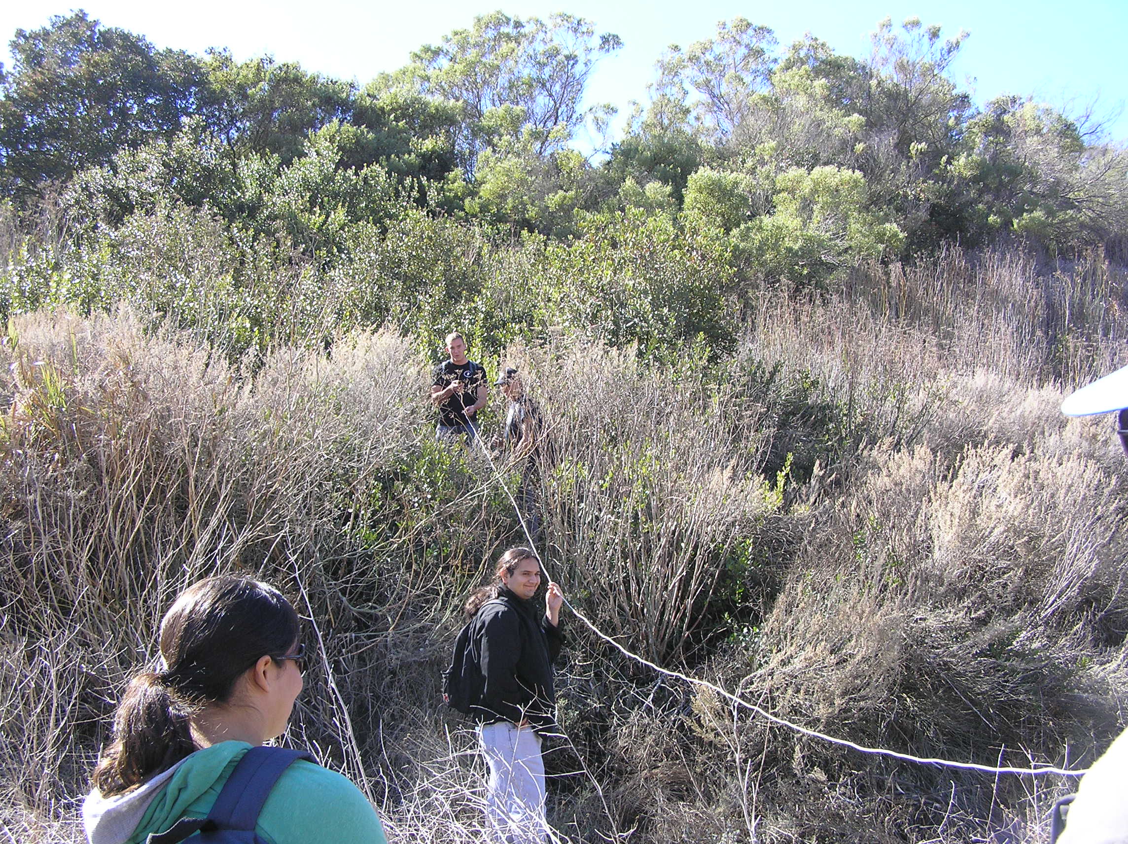
Plant identification can be very time-consuming. You need to prepare for the trip by learning many of the plants you are likely to encounter ahead of time, so that this part goes faster in the field. You can do this by acquiring a species list for the area. These are sometimes published for parks. You can also use the "What Grows Here?" web site provided by Calflora: https://www.calflora.org/entry/wgh.html to generate a suitable list, and then using the site to learn a bit about each species (Lab 3 will give you practice in using Calflora's WGH). You should also bring along a floristic key or access an online key (which depends on your cell phone having access in the area and struggling with sunlight...). Labs 4 and 5 will give you practice in working through a key.

Sometimes, you just plain can't identify a plant. In that situation, comment in the field notebook, describing the point on the transect line it was found, giving it an identification name (e.g., "Unknown shrub #2"), describing its appearance, taking a photograph of it, and taking a small sample of it (put it in a plastic bag, and label the bag with the ID and transect and transect point). Back in the lab or at home, you can try to identify it by close examination and trying to key it out there.

So, that's the general idea. I thought I'd have you try it out using a map in the comfort of a computer lab or, during COVID-19, of your home lab, so you can focus just on the statistical sampling aspect.

Getting Your Data

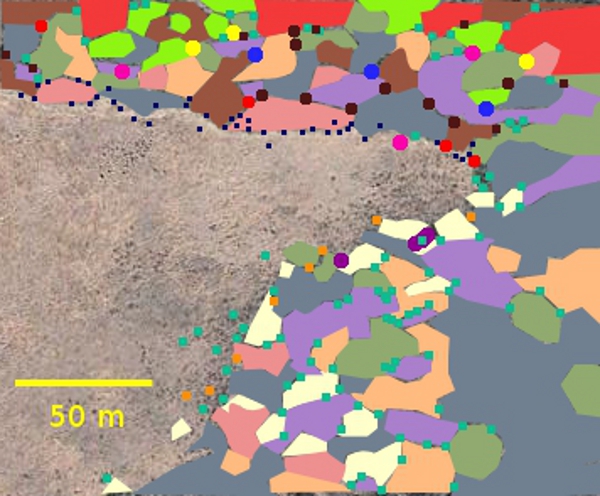
Here is your field site, showing an area of California sage scrub (CSS) where it bounds an area covered with exotic-dominated annual grassland. The image was taken in late summer 2007, so the grassland vegetation is dead and the grass unidentifiable. The CSS was crudely mapped based on sample data taken in 2009 and 2010. Each of the colored patches represents an area that is largely dominated by one of eighteen different species common in this western Santa Monica Mountains area.

• Map: https://home.csulb.edu/~rodrigue/geog330/labs/LJVtransectlabcropped.jpg

• Key to the color codes identifying species: https://home.csulb.edu/~rodrigue/geog330/labs/LJVtransectmapkey.pdf

Notice that the CSS looks somewhat different along the two major sections of this CSS-grassland boundary, a different mix of species in common and some species that are found in one area and not the other. Eyeballing this map, where would you separate the two regions of CSS and why?

One of these boundaries has been stable for several decades, showing hardly any change from one remote sensing image to the next. This is a "stable boundary." If you look close, you'll see that the boundary is pretty sharp and there's a kind of bare area about a meter or two wide along much of it. Which boundary on the map are we talking about here?

The other boundary has shifted over the decades, with CSS making inroads into the grassland. The boundary there is more uneven: More CSS species can be seen out past the boundary. This is an "ecotone" type of boundary: less sharp, harder to delineate. This is the "recovering boundary" (from the point of view of the CSS and people trying to restore it).

Let's use transecting to see if we can characterize the "personality" of the two CSS patches and find out if there is some difference in the mix of CSS species in the area of expansion versus the more stagnant areas. Given that CSS has declined sharply in Southern California over the last couple of centuries and that many CSS restoration projects are not successful, it is heartening to find that CSS can restore itself in certain situations. The race is on to find out what those situations are, to help conservancies make use of CSS self-restoration. It would also be helpful to see if there is a process of succession here, with certain species likelier to lead the way into the grassland, CSS pioneers or the reclamation vanguard.

Your transect tapes are 40 m long (you can measure them against the scale bar on the map). We'll sample along them every 10 m, yielding 5 sample identifications per transect. A dozen or so transects, half in the CSS behind the stable boundary and half in the CSS behind the recovering boundary, would produce at least 60 sample identifications, or over 30 per boundary type. That would be a workable sample size for statistical purposes.

Let's aim for samples that are as unbiased as possible and from transects that don't cross one another (don't want to double-dip). A good sampling approach in this situation is systematic random sampling, where we pick a starting point as randomly as possible and then run our lines parallel to one another an equal interval apart from that point. We'll need an orientation.

Picking an orientation randomly isn't going to work here, because the two boundaries are oriented at roughly right angles to one another. Going straight in from one boundary would mean you were running parallel to the opposite boundary type. So, let's arbitrarily pick a compromise orientation that will create angled transects but roughly similarly angled in each patch of CSS. Let's aim for about 40°, running from the northwest to the southeast.

Here is a map of six parallel transects that cover both the recovering (southeast) and the stable (north)boundaries at a similar angle of entry into the shrubbery: https://home.csulb.edu/~rodrigue/geog330/labs/LJVtransectlabtransects.jpg. The lines fill that portion of each boundary region that can accommodate a 40 m transect tape.

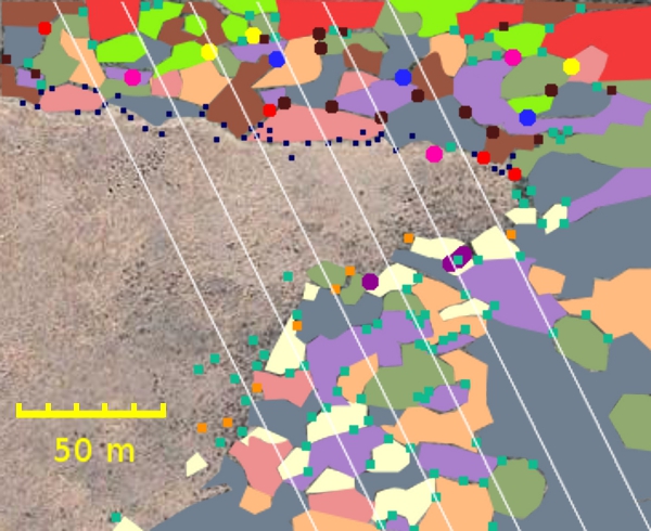
Take the one that, in the upper left, allows at least a 40 m transect to go from the stable border up into the CSS there without crossing the edge of the map. Label that line S1. The one in the stable CSS that's 20 m east of it is labelled S2, and so forth. Go back to S1 and follow that line south until you hit the recovering boundary. Start transect R1 there. Label the next one R2 and so forth until you reach the last complete line to the east.

I will assign each student one of these twelve transects to work on. Each transect should wind up covered by at least two students.

You need a virtual transect tape, which you'll fake out in your home lab. First, get a card or piece of paper with a straight edge. Align the edge of that card or paper on the computer screen (or a print out) with the yellow scale bar. Carefully mark your card or paper at 50 m from its edge. Now, carefully divide that 50 m into five equal-width sections, marking the edge of the sections (4 more marks) with the tick marks on the scale. Label the marks 0, 10, 20, 30, and 40. Voilà! -- virtual transect lines.

Doing Your Transect

For each transect, align your marked card EXACTLY along the transect line you were assigned on the map. At each tick mark on the card, identify the plant at precisely that location. To make the identifications, compare the color of the patch with the color key. It's designed so the color swatch is right on the edge, so you may be able to move that edge of the image in one browser window with the map in a second browser window to do your comparisons if you can't match the colors otherwise. If you have a color printer, that might be another way to match the colors on the key with the colors on the map.

Then, once you're pretty sure which species is at which tick mark, fill out the data entry spreadsheet. Using the Raw Data tab, enter the Latin names for each of your five identifications. The 0 entry should be for the plant RIGHT on the boundary with the grassland, while the #4 entry is for the plant identified 40 meters out in the farthest reaches of the shrubbery. Be aware that there may be some judgment call situations. If your sampling point is right where two or three species meet, resolve it by the one that seems closest to dominating your point. Make sure to label the sheet with the name of the transect you were assigned (R1, S3, or whatever) and your own name.

Now, click on the Counts tab to arrange your data a different way. You will notice that very few species were "captured" on your transect, and you may have gotten more than one occurrence of a given species. Look up your transect in the Counts tab (recovering boundary transects are in the pink block of columns and stable boundary transects are in the green block of columns). Count up how many of each species turned up in your transect and put the counts in the appropriate row for each species. Check your work by making sure the automated sum is exactly 5. Make sure your name is on the sheet.

Now, turn that spreadsheet in, ideally saved as Lab1dataentryYourLastName.ods. Put it in the Dropbox for Lab 1 on BeachBoard. Then, my work begins: I'll collect all the transects and create a master spreadsheet with all the data filled in and put it on the course home page for you to download for the next step. .

Comparing Boundary Types

In this phase of the lab, we'll figure out which species are found in which boundary type. Some species may be found in both the stable and the recovering patches, while others may be found only in one or the other type of boundary patch.

Download https://home.csulb.edu/~rodrigue/geog330/labs/Lab1StableRecoveringDataF20.ods when I let you know it's done.

Download the consolidated classification sheet, https://home.csulb.edu/~rodrigue/geog330/labs/Lab1ConsolidationF20.ods. In its upper table, count up the number of times each species was found in the recovering boundary and how many times it was found in the stable boundary. Once that's done, classify each species as B for found in both kinds of patch; S for found ONLY in the stable patch, and R for found only in the recovering patch. Sum up how many individuals of each species were found in the Totals column. Also, sum up the number of plants at the bottom of the Stable and Recovering columns, too.

In the lower table, you're going to turn the numbers into simple presence-absence data by converting any number in the upper table into an X in the lower table (and bring down the B, S, and R classifications into that lower table, too. For each species, count the Xs and put that total in the right column: It should only be 0, 1, or 2.

With presence-absence data, we can now calculate alpha, beta, and gamma diversities. Alpha diversity is the species richness in one small patch of a landscape (here the stable or the recovering boundary patches). Gamma diversity is the species richness for the whole landscape of patches. Beta diversity is something else: Instead of measuring species richness, it counts up contrasts between patches, or the species NOT shared between them.

So, count the X's in the Stable column: That is the alpha diversity for that patch. Count the Xs in the Recovering patch for its alpha diversity. Count all the Bs, Ss, and Rs in that column: That is the overall gamma diversity for the California sage scrub (CSS) in that part of La Jolla Valley. Now, if you count only the number of 1s in the rightmost totals column, you will have the beta diversity for the comparison of stable and recovering boundary patches. Beta diversity is a measure of the contrast between patches, counting only those species that are found in only one patch, not both.

Transfer your answers for alpha, beta, and gamma diversities to the answer sheet, https://home.csulb.edu/~rodrigue/geog330/labs/Lab1AnswerSheet.ods (and type in your name). Upload both the consolidated worksheet and the answer sheet to the Lab 1 Dropbox in BeachBoard. And that's a wrap for the virtual transect lab.

Lab deliverables (3 spreadsheets):

• Your transect data:
  • Your transect data entry form, properly labelled by transect name and including your name (always nice to get credit!). This goes on the Raw Data tab for y our data entry spreadsheet.
  • On the Counts tab of the same data entry spreadsheet, locate your transect and, using your raw data, count up the number of times a given species was found on your transect line. Enter your counts in the correct column and put your name on the spreadsheet.
  • The spreadsheet with its filled out tabs should then be saved (maybe as Lab1dataYourLastName.ods) and then uploaded to the BeachBoard Dropbox for Lab 1.
• I will put together a master spreadsheet with each of your transects on it and get it back to you. Then, you can work on classifying each species found out there by its presence or absence in the recovering boundary (southeast patch) and/or the stable boundary (north patch).
  • Turn in the consolidated classification spreadsheet (with your name on it) to the BeachBoard Dropbox
  • You can then figure out the alpha, beta, and gamma diversities of the field site and enter those in the diversity answer sheet and upload that to BeachBoard

| GEOG/ES&P 330 Home | Dr. Rodrigue's Home | Geography Home | ES&P Home | EMER Home |

| CSULB Home | BeachBoard | MyCSULB | Campus Search | Library |

Document maintained by Dr. Rodrigue
First placed on web: 08/27/15
Last revision: 08/14/20