Dr. Rodrigue, Quant. Methods, Lab 2

Geography 200: INTRODUCTION TO RESEARCH METHODS FOR GEOGRAPHERS

Dr. Rodrigue

Graded Lab 2: BASIC DATA DESCRIPTION AND PRESENTATION

EXERCISE A: Basic Concepts

Levels of Measurement:

It is very important to understand the concept of levels of measurement, as it affects the kinds of descriptive statistics and tests that you can legitimately apply to your data and even the most basic choice of data graphing. Data can be characterized as nominal, ordinal, or scalar, and each of these has a couple of subtypes. After reading chapter 2 in ML & M and reviewing your lecture notes, identify the following data sets as (a) binary; (b) other nominal; (c) ordinal: strongly ordered; (d) ordinal: weakly ordered; (e) interval; or (f) ratio. Briefly defend your selection.


 1.  Survey respondents' genders __________________________________________

 2.  Temperature in degrees centigrade ____________________________________

     ______________________________________________________________________ 

 3.  Standard Industrial Classification (SIC)#3714_________________________

     ______________________________________________________________________
     (careful here -- this one is tricky -- you need to visit this link)


 4.  Elevations above sea level in meters on a topo sheet _________________

     ______________________________________________________________________ 

 5.  Places  Rated Almanac, individually ranking more than 400  communities 
     on each of several axes of livability 

     ______________________________________________________________________ 

 6.  Rodrigue's classification of 600 archaeological sites in the Near East 
     of  20,000  years ago to 5,000 years ago as Upper  Palaeolithic,  Epi-
     Palaeolithic, Mesolithic, or Neolithic, based on general technological 
     level) 
             ______________________________________________________________

 7.  Precipitation  receipt  in  centimeters at  each  weather  station  in 
     California
                ___________________________________________________________

     ______________________________________________________________________ 


 8.  Yes-no answers on a questionnaire  ___________________________________

 9   Yes-no-I don't know answers on a questionnaire _______________________

     ______________________________________________________________________ 


10.  Weather  stations   classified  by average   annual  precipitation  in 
     centimeters into <25 cm; 25-99 cm; and > 100 cm 

     ______________________________________________________________________

Recognizing Graphic Types:

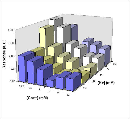
The links below take you to a variety of graphs. Identify the following graphic representations directly on the handout as (a) number line; (b) histogram; (c) bar chart; (d) frequency polygon; (e) ogive; (f) scatterplot; (g) X-Y fitted curve; and (h) 3-D histogram.

Grades by percentage of students in class: ________

Occupation and use of therapy: ________

Timber exports by year: ________

Test marks: ________

Red wine and age at death: ________

________

                                   x
                       x           x  x     x  
           x     x     x     x  x  x  x  x  x     x  x
      x    x  x  x     x  x  x  x  x  x  x  x     x  x  x     x     
     ___________________________________________________________
     66 67 68 69 70 71 72 73 74 75 76 77 78 79 80 81 82 83 84 85
                   student scores on midterm

Diameter at breast height of several Australian tree species and density of stems per hectare: ________
Calcium and potassium response of Fabrea salina: ________
Time since dose and blood concentration: ________
Height and weight: ________

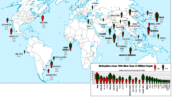
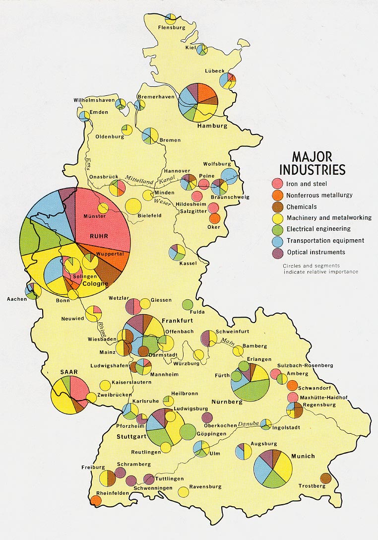
Recognizing Basic Map Types:

Examine the following maps. Identify each map as one of the following: (a) choropleth map; (b) isoline map; (c) dot map; (d) graduated point symbol map.

Size of population in world metropolitan areas of more than 10 million in 1985 and 2025: ________
% of water withdrawals from surface water sources: ________
Mean maximum temperatures, 12 month period: ________
Hogs in North Carolina: ________
Size of West German cities and percentage of their industrial base in particular industries: ________

EXERCISE B: Application

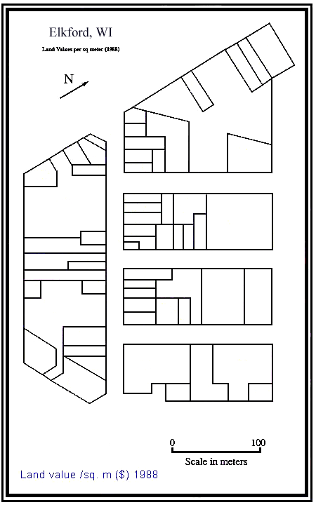
Data Set:

The land values map shows a somewhat imaginary town's commercial core, with each lot marked and its going land value per square meter. After reading chapter 3 in ML & M (and maybe Chapter 2 of HyperStat Online), answer the following questions. Show the results of your calculations to TWO decimal places of accuracy (even if the answer is an even number or when the second digit after the decimal point is a zero, e.g., 2.00 or 3.50, instead of 2 or 3.5). I'll grade you down a bit if you don't round to two decimal places!

 1.  Convert   the land values into a ranked array.  It's easiest   to   enter      
     each   value into your spreadsheet and then ask it to arrange   them   by      
     ascending   or descending order.  That done, you can pretty it   up   and 
     print it.  You should find a way to get this all on one page, perhaps by 
     printing different sections of the array in separate rows or columns 

 2.  Compute the mean land value for Elkford:   ______________________________

 3.  Construct  a  number line showing every single value, highest to  lowest, 
     putting  (a)  mark(s)  by any values that appear in  your  ranked  array, 
     corresponding   to  the  number  of  Elkford  parcels  that   have   that 
     value/m².  To save on paper, you should find a way to get the 
     whole number line on one sheet, perhaps by breaking it up into sections 
     and showing the sections as parallel vertical or horizontal lines. Other-
     wise, you will waste several pages!

                                                ______________________________

 4.  What is the modal land value?              ______________________________

 5.  Determine the median land value:           ______________________________

 6.  What would be the interquartile range?

     From ______________________________   to   ______________________________

 7.  Construct   a  histogram for these values, thinking  about   the   issues      
     raised  in  ML & M 2.4 (chapter 2, section 4). It is okay to  do  this  by 
     hand, but neatness is important.

 8.  Construct   a  choropleth map of land values in Elkford,  so  that   the      
     "high   and  low  rent  districts"  are  easily apparent.   Be  sure   to 
     contemplate  the issues above (2.4 in ML & M)  and their figures 2.3   and      
     2.4. It is okay to do this (neatly) by hand on the blank map provided.

     Use this blank map. 

 9.  Construct a frequency polygon, just to say you know how. By hand is okay.

10.  Construct an ogive, too, while you're at it. By hand is okay.

11.  What is the standard deviation?            ______________________________

12.  What is the variance?                      ______________________________

13.  Calculate Pearson's Skewness:              ______________________________

14.  Briefly interpret the skewness of this particular distribution

     _________________________________________________________________________

     _________________________________________________________________________


15.  Calculate kurtosis, using this formula (don't forget the -3 at the end):
     



16.  Briefly interpret the kurtosis value ____________________________________

     _________________________________________________________________________

==========