A possitive charged rod
H.Tahsiri
A thin non-conducting rod of finite length L carries a total charge
Q,spread uniformly along it.
a) Find the components of the electric fields.
b) find y-component of the electric field for ( L-> infinity >> y ) by two different methods
i) by taking the limit. ii) by direct integration.
Enter the above equations in the Mathematica notebook
as follow.
Ey=lamda 1/(4Pi eps0) y Integrate[1/(x^2+y^2)^(3/2),{x,-L/2,L/2}]


               L lamda
     ---------------------------
                       2      2
     2 eps0 Pi y Sqrt[L  + 4 y ]
Ex=lamda 1/(4Pi eps0) y Integrate[x/(x^2+y^2)^(3/2),{x,-L/2,L/2}]


     0
EylargeL=Limit[Ey,L->Infinity]


        lamda
     -----------
     2 eps0 Pi y

EylargeL=lamda 1/(4Pi eps0) y Integrate[1/(x^2+y^2)^(3/2),
     {x,-Infinity,Infinity}]


        lamda
     -----------
     2 eps0 Pi y
Plot the electric field lines in the z-y plane.
This problem has cylindrical symmetry with respect to the x-axis
at all points in the yz plane
of radius y=r from the charged rod.
Enter the z and the y components of the electric field as follow.
Ezcompnt=lamda L z/(2 Pi eps0 (z^2+y^2) Sqrt[L^2+4(z^2+y^2)])


                     L lamda z
     ------------------------------------------
                 2    2        2       2    2
     2 eps0 Pi (y  + z ) Sqrt[L  + 4 (y  + z )]
Eycompnt=lamda L y/(2 Pi eps0 (z^2+y^2) Sqrt[L^2+4(z^2+y^2)])


                     L lamda y
     ------------------------------------------
                 2    2        2       2    2
     2 eps0 Pi (y  + z ) Sqrt[L  + 4 (y  + z )]
given={eps0->1/(4N[Pi] 9 10^9),L=1;Q=10^(-6);lamda->Q/L};
Efield={Ezcompnt,Eycompnt}/.given//N


                  18000. z                           18000. y
     {---------------------------------, ---------------------------------}
        2    2                 2    2      2    2                 2    2
      (y  + z ) Sqrt[1. + 4. (y  + z )]  (y  + z ) Sqrt[1. + 4. (y  + z )]
<<Graphics`PlotField` (* This command will load the plotting
routin for the vector field *)

Efieldplot=PlotVectorField[Efield,{z,-.1,.1},{y,-.1,.1},
PlotPoints->8,ColorFunction->None];


Clear[given,L]
V=lamda/(4Pi eps0) Integrate[1/(x^2+y^2)^(1/2),{x,-L/2,L/2}]

                            2                        2
                 -L        L     2         L        L     2
     lamda (-Log[-- + Sqrt[-- + y ]] + Log[- + Sqrt[-- + y ]])
                 2         4               2        4
     ---------------------------------------------------------
                             4 eps0 Pi
potential=V/.y^2->z^2+y^2

                            2                             2
                 -L        L     2    2         L        L     2    2
     lamda (-Log[-- + Sqrt[-- + y  + z ]] + Log[- + Sqrt[-- + y  + z ]])
                 2         4                    2        4
     -------------------------------------------------------------------
                                  4 eps0 Pi
given={eps0->1/(4Pi 9 10^9),L=1;Q=10^(-6);lamda->Q/L};
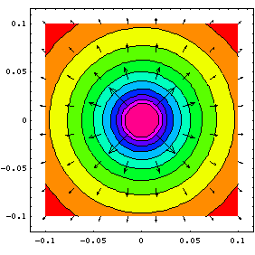
pplot=ContourPlot[potential/.(given//N),{z,-.1,.1},{y,-.1,.1},
PlotPoints->26,ColorFunction->Hue]

ez=-D[potential,z]//Simplify//Together


                      lamda z
     -----------------------------------------
                 2    2              2      2
     2 eps0 Pi (y  + z ) Sqrt[1 + 4 y  + 4 z ]
ey=-D[potential,y]//Simplify//Together


                      lamda y
     -----------------------------------------
                 2    2              2      2
     2 eps0 Pi (y  + z ) Sqrt[1 + 4 y  + 4 z ]
together=Show[{pplot,Efieldplot}];