Back Propagation Lab
Background
The purpose of this lab is to familiarize you with the backpropagation
simulator, convince you that backpropagation can be used to train networks
to do relatively difficult tasks, and to give you some idea of what the equations
that define the system actually mean (i.e., what the system is really supposed
to be doing).
Why Three Layers?
Original work on connectionist-type systems was done as early as the 1940's.
In 1943 Warren McCulloch and Walter Pitts wrote their A Logical Calculus
of the Ideas Immanent in Nervous Activity. Though interest in connectionist
systems flagged, it was revived in the 1960's. Among the major contributions
was Frank Rosenblatt's Principles of Neurodynamics, in which he defined
systems called perceptrons and proved a number of theories about them. One
theory Rosenblatt proved was that perceptrons could learn to do any problem
that one could program it to do (i.e., build it to do). Perceptrons could
do many interesting things, but they also failed to solve problems. In 1969
Marvin Minsky and Seymour Papert wrote a book, Perceptrons, in which
they rigorously proved that perceptrons could not solve any problems that
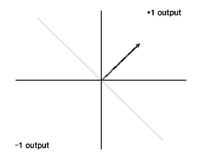
were not linearly seperable. That is, they couldn't solve problems in which
the correct division of the weightspace is not a plane between the one possibility
and another.
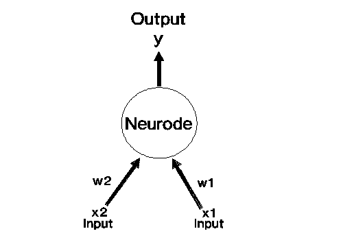
Typical Perceptron Configuration

Partition of Weightspace for Linearly
Separable Problem
Minsky and Papert took their result to apply to all such networks since
they had proven it for one- and two-layer networks and since they thought
that no learning procedure could be developed for three layer networks.
(Why assume this? They knew that error in the output was used to change
weights in such systems and they didn't think there was any way to calculate
error for the middle layer.) However, as we will see, there is a way to estimate error (and hence change
weights) in three layer systems and they are not subject to the limitations
of perceptrons and similar networks.
Training (Generally)
During the training period, the network works in a two-step sequence. First, input is given to the system and it passes through to the output layer. Second, the error in the output is determined by comparing the system's output to the desired output. If the error is higher than the learning threshold, then the system works backward to reset weights in light of the error.
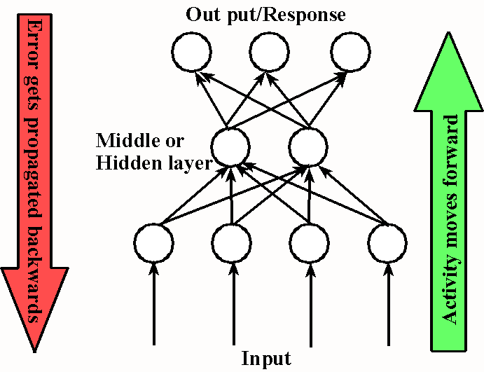
Input/Output for a Given Neurode
The input/output relations for a neurode are different for three layer
systems. The input (I) is calculated as the sum of the weighted input from
all the neurodes in the previous level.

Input/Output for a Given Neurode
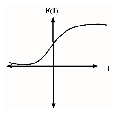
The output of the neurode is determined by what is sometimes called a
"squashing function". A function that generates output in a way in which
it is easy to take the derivative of the output given the input (determine
the change of output given the change of input). The most common function
is the sigmoid function:

Learning and Weight Change
The basic weight change equation tells us to change the weight between
two neurodes, i and j, by the output for the neurode, i, multiplied by the
error and the learning constant:

To find the amount we need to change the weight, we need to figure out
the error. For the output neurodes, that is easy:

But for the middle layer neurodes, we have to calculate the error by multiplying rate of output change given input change for the neurode, i, by the sum of the error for the each output neurode, j, times the weight between that neurode, j, and the middle neurode, i:

In other words, as a middle neurode, the weight of your connection to a given output neurode will be changed by the amount of activity you contribute per unit of input multiplied by the product of your old weight and the error for that output neurode (how much input to the ouput neurode you will likely have multiplied by how much of the error at the output neurode was your fault).
